The modem module implements a set of (mod)ulation/(dem)odulation schemes for encoding information into signals. For the analog modems, samples are encoded according to frequency or analog modulation. For the digital modems, data bits are encoded into symbols representing carrier frequency, phase, amplitude, etc. This section gives a brief overview of linear modulation schemes available in liquid , and provides a brief description of the interfaces. For non-linear digital modulation, see the documentation on GMSK , CP-FSK , and FSK .
Modulation Types∞
The modem object realizes the linear digital modulation library in which the information from a symbol is encoded into the amplitude and phase of a sample. The modem structure implements a variety of common modulation schemes, including (differential) phase-shift keying, and (quadrature) amplitude-shift keying. The input/output relationship for modulation/demodulation for the modem object is strictly one-to-one and is independent of any pulse shaping, or interpolation.
In general, linear modems demodulate by finding \(\hat{s}\) , the closest of \(M\) symbols in the set \(\mathcal{S}_M = \{s_0,s_1,\ldots,s_{M-1}\}\) to the received symbol \(r\) , viz
$$ \hat{s} = \underset{s_k \in \mathcal{S}_M}{\arg\min} \bigl\{ \| r - s_k \| \bigr\} $$For arbitrary modulation schemes a linear search over all symbols in \(\mathcal{S}_M\) is required which has a complexity of \(\mathcal{O}(M^2)\) ; however one may take advantage of symmetries in certain constellations to reduce this to \(\mathcal{O}(\log(M))\) .
Table [tab-modem-schemes]. Linear Modulation Schemes Available in liquid
| Modulation Scheme | Bits/Symbol | Description |
| LIQUID_MODEM_UNKNOWN | - | unknown/unsupported scheme |
| LIQUID_MODEM_PSK{2,4,8,16,32,64,128,256} | 1-8 | phase-shift keying |
| LIQUID_MODEM_DPSK{2,4,8,16,32,64,128,256} | 1-8 | differential phase-shift keying |
| LIQUID_MODEM_ASK{2,4,8,16,32,64,128,256} | 1-8 | amplitude-shift keying |
| LIQUID_MODEM_QAM{4,8,16,32,64,128,256} | 2-8 | quadrature amplitude-shift keying |
| LIQUID_MODEM_APSK{4,8,16,32,64,128,256} | 2-8 | amplitude/phase-shift keying |
| LIQUID_MODEM_BPSK | 1 | binary phase-shift keying |
| LIQUID_MODEM_QPSK | 2 | quaternary phase-shift keying |
| LIQUID_MODEM_OOK | 1 | on/off keying |
| LIQUID_MODEM_SQAM32 | 5 | "square" 32-QAM |
| LIQUID_MODEM_SQAM128 | 7 | "square" 128-QAM |
| LIQUID_MODEM_V29 | 4 | V.29 star modem |
| LIQUID_MODEM_ARB16OPT | 4 | optimal 16-QAM |
| LIQUID_MODEM_ARB32OPT | 5 | optimal 32-QAM |
| LIQUID_MODEM_ARB64OPT | 6 | optimal 64-QAM |
| LIQUID_MODEM_ARB128OPT | 7 | optimal 128-QAM |
| LIQUID_MODEM_ARB256OPT | 8 | optimal 256-QAM |
| LIQUID_MODEM_ARB64VT | 6 | Virginia Tech logo |
| LIQUID_MODEM_ARB | 1-8 | arbitrary signal constellation |
Interface∞
- modem_create(scheme) creates a linear modulator/demodulator modem object with one of the schemes defined in [ref:tab-modem-schemes] .
- modem_recreate(q,scheme) recreates a linear modulator/demodulator modem object q with one of the schemes defined in [ref:tab-modem-schemes] .
- modem_create_arbitrary(*table,M) creates a generic arbitrary modem ( LIQUID_MODEM_ARB ) with the \(M\) -point constellation map defined by the float complex array table . The resulting constellation is normalized such that it is centered at zero and has unity energy. Note that \(M\) must be equal to \(2^m\) where \(m\) is an integer greater than zero.
- modem_destroy(q) destroys a modem object, freeing all internally-allocated memory.
- modem_print(q) prints the internal state of the object.
- modem_reset(q) resets the internal state of the object. This method is really only relevant to LIQUID_MODEM_DPSK (differential phase-shift keying) which retains the phase of the previous symbol in memory. All other modulation schemes are memoryless.
- modem_gen_rand_sym(q) generates a random integer symbol in \(\{0,M-1\}\) .
- modem_get_bps(q) returns the modem's modulation depth (bits/symbol).
- modem_modulate(q,symbol,*x) modulates the integer symbol storing the result in the output value of \(x\) . The input symbol value must be less than the constellation size \(M\) .
- modem_demodulate(q,x,*symbol) finds the closest integer symbol which matches the input sample \(x\) . The exact method by which liquid performs this computation is dependent upon the modulation scheme. For example, while LIQUID_MODEM_QAM4 , and LIQUID_MODEM_PSK4 are effectively equivalent (four points on the unit circle) they are demodulated differently.
- modem_demodulate_soft(q,x,*symbol,*softbits) demodulates as with modem_demodulate() (see above) but also populates the\(m\) -element array of unsigned char as an approximate log-likelihood ratio of the soft-decision demodulated bits (see [ref:section-modem-digital-soft] ).
- modem_get_demodulator_sample(q,*xhat) returns the estimated transmitted symbol, \(\hat{x}\) , after demodulation.
- modem_get_demodulator_phase_error(q) returns an angle proportional to the phase error after demodulation. This value can be used in a phase-locked loop (see [ref:section-nco-pll] ) to correct for carrier phase recovery.
- modem_get_demodulator_evm(q) returns a value equal to the error vector magnitude after demodulation. The error vector is the difference between the received symbol and the estimated transmitted symbol, \(e = r - \hat{s}\) . The magnitude of the error vector is an indication to the signal-to-noise/distortion ratio at receiver.
While the same modem structure may be used for both modulation and demodulation for most schemes, it is important to use separate objects for differential-mode modems (e.g. LIQUID_MODEM_DPSK ) as the internal state will change after each symbol. It is usually good practice to keep separate instances of modulators and demodulators. This holds true for most any encoder/decoder pair in liquid . An example of the modem interface is listed below.
#include <liquid/liquid.h>

int main() {
    // create mod/demod objects
    modulation_scheme ms = LIQUID_MODEM_QPSK;

    // create the modem objects
    modem mod   = modem_create(ms); // modulator
    modem demod = modem_create(ms); // demodulator
    modem_print(mod);

    unsigned int sym_in;    // input symbol
    float complex x;        // modulated sample
    unsigned int sym_out;   // demodulated symbol

    // ...repeat as necessary...
    {
        // modulate symbol
        modem_modulate(mod, sym_in, &x);

        // demodulate symbol
        modem_demodulate(demod, x, &sym_out);
    }

    // destroy modem objects
    modem_destroy(mod);
    modem_destroy(demod);
}
Gray coding∞
In order to reduce the number of bit errors in a digital modem, all symbols are automatically Gray encoded such that adjacent symbols in a constellation differ by only one bit. For example, the binary-coded decimal (BCD) value of 183 is 10110111 . It has adjacent symbol 184 ( 10111000 ) which differs by 4 bits. Assume the transmitter sends 183 without encoding. If noise at the receiver were to cause it to demodulate the nearby symbol 184, the result would be 4 bit errors. Gray encoding is computed to the binary-coded decimal symbol by applying an exclusive OR bitmask of itself shifted to the right by a single bit.
        10110111    bcd_in (183)        10111000    bcd_in (184)
        .1011011    bcd_in >> 1         .1011100    bcd_in >> 1
xor :   --------                        --------
        11101100    gray_out (236)      11100100    gray_out (228)
Notice that the two encoded symbols 236 ( 11101100 ) and 228 ( 11100100 ) differ by only one bit. Now if noise caused the receiver were to demodulate a symbol error, it would result in only a single bit error instead of 4 without Gray coding.
Reversing the process (decoding) is similar to encoding but slightly more involved. Gray decoding is computed on an encoded input symbol by adding to it (modulo 2) as many shifted versions of itself as it has bits. In our previous example the receiver needs to map the received encoded symbol back to the original symbol before encoding:
        11101100    gray_in (236)       11100100    gray_in (228)
        .1110110    gray_in >> 1        .1110010    gray_in >> 1
        ..111011    gray_in >> 2        ..111001    gray_in >> 2
        ...11101    gray_in >> 3        ...11100    gray_in >> 3
        ....1110    gray_in >> 4        ....1110    gray_in >> 4
        .....111    gray_in >> 5        .....111    gray_in >> 5
        ......11    gray_in >> 6        ......11    gray_in >> 6
        .......1    gray_in >> 7        .......1    gray_in >> 7
xor :   --------                        --------
        10110111    gray_out (183)      10111000    gray_out (184)
There are a few interesting characteristics of Gray encoding:
- the first bit never changes in encoding/decoding
- there is a unique mapping between input and output symbols
It is also interesting to note that in linear modems (e.g. PSK), the decoder is actually applied to the symbol at the transmitter while the encoder is applied to the received symbol at the receiver. In liquid , Gray encoding and decoding are computed with the gray_encode() gray_decode() methods, respectively.
LIQUID_MODEM_PSK (phase-shift keying)∞
With phase-shift keying the information is stored in the absolute phase of the modulated signal. This means that each of \(M=2^m\) symbols in the constellation are equally spaced around the unit circle.
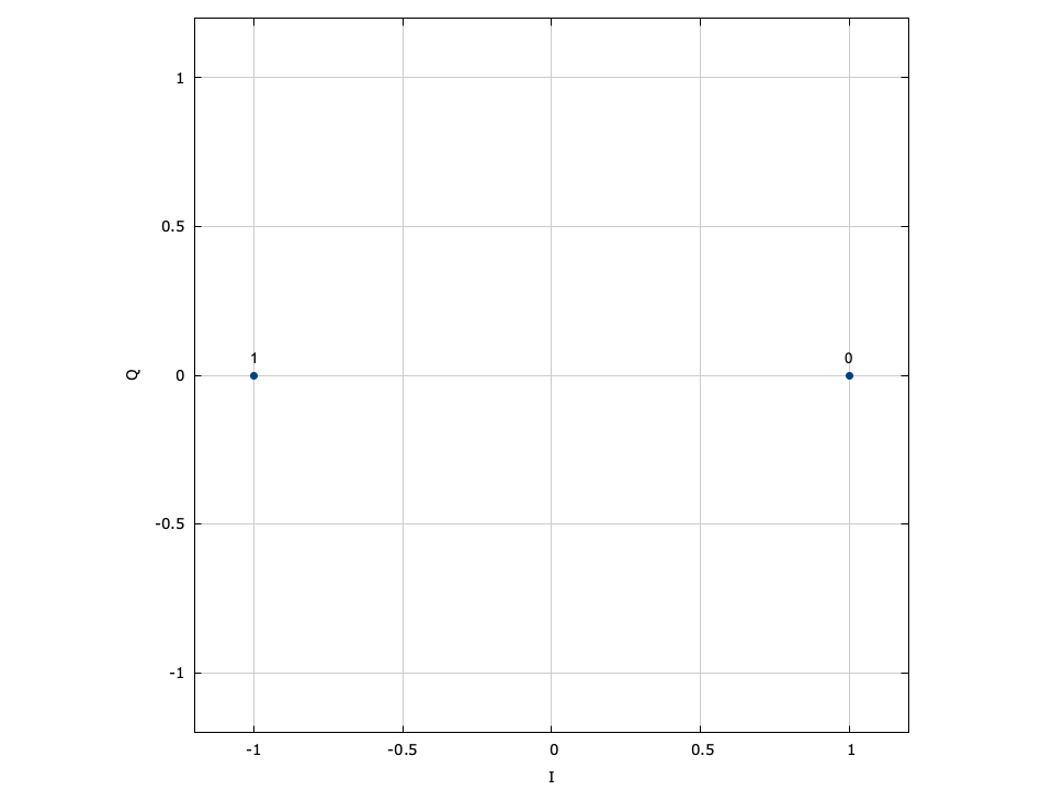
Figure [fig-modem-psk-2]. 2-PSK (generic BPSK)
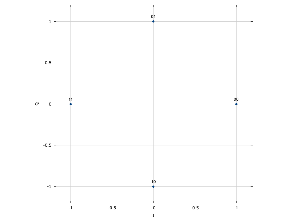
Figure [fig-modem-psk-4]. 4-PSK (generic QPSK)
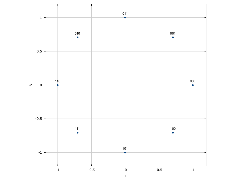
Figure [fig-modem-psk-8]. 8-PSK

Figure [fig-modem-psk-16]. 16-PSK
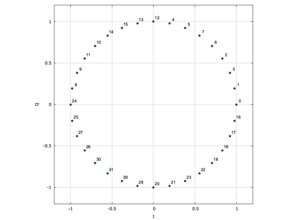
Figure [fig-modem-psk-32]. 32-PSK
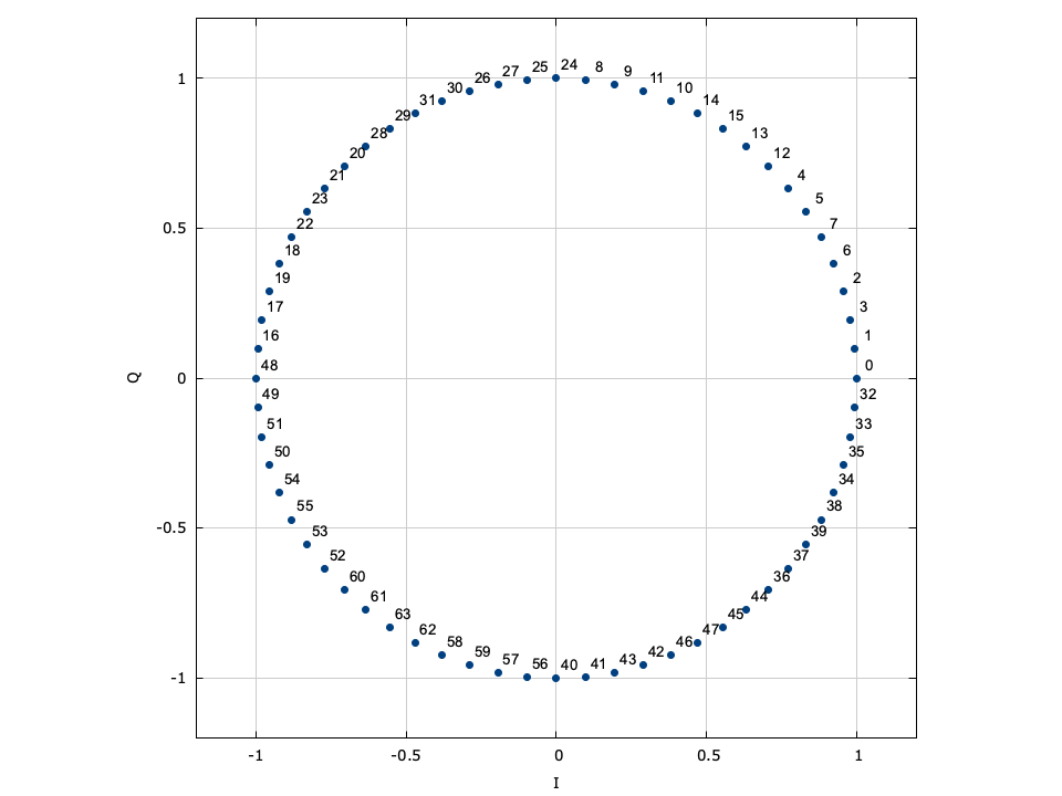
Figure [fig-modem-psk-64]. 64-PSK
Figure [fig-modem-psk]. Phase-shift keying (PSK) modem constellation map. Note that BPSK and QPSK are customized implementations of 2-PSK and 4-PSK. While only PSK up to \(M=64\) are shown, liquid supports up to 256-PSK.
[ref:fig-modem-psk] depicts the constellation of PSK up to \(M=16\) with the bits gray encoded. While liquid supports up to \(M=256\) , values greater than \(M=32\) are typically avoided due to error rates for practical signal-to-noise ratios. For an \(M\) -symbol constellation, the \(k^{th}\) symbol is
$$ s_k = e^{j 2 \pi k/M} $$where \(k \in \{0,1,\ldots,M-1\}\) . Specific schemes include BPSK (\(M=2\) ),
$$ s_k = e^{j \pi k} = \begin{cases} +1 & k=0 \\ -1 & k=1 \end{cases} $$and QPSK (\(M=4\) )
$$ s_k = e^{j\left(\pi k/4 + \frac{\pi}{4}\right)} $$Demodulation is performed independent of the signal amplitude for coherent PSK.
LIQUID_MODEM_DPSK (differential phase-shift keying)∞
Differential PSK (DPSK) encodes information in the phase change of the carrier. Like regular PSK demodulation is performed independent of the signal amplitude; however because the data are encoded using phase transitions rather than absolute phase, the receiver does not have to know the absolute phase of the transmitter. This allows the receiver to demodulate incoherently, but at a quality degradation of 3dB. As such the \(n^{th}\) transmitted symbol \(k(n)\) depends on the previous symbol, viz
$$ s_k(n) = \exp\left\{ \frac{ j 2 \pi \Bigl(k(n) - k(n-1)\Bigr) } { M } \right\} $$LIQUID_MODEM_APSK (amplitude/phase-shift keying∞
Amplitude/phase-shift keying (APSK) is a specific form of quadrature amplitude modulation where constellation points lie on concentric circles. The constellation points are further apart than those of PSK/DPSK, resulting in an improved error performance. Furthermore the phase recovery for APSK is improved over regular QAM as the constellation points are less sensitive to phase noise. This improvement comes at the cost of an increased computational complexity at the receiver. Demodulation follows as a two-step process: first, the amplitude of the received signal is evaluated to determine in which level ("ring") the transmitted symbol lies. Once the level is determined, the appropriate symbol is chosen based on its phase, similar to PSK demodulation. Demodulation of APSK consumes slightly more clock cycles than the PSK and QAM demodulators.
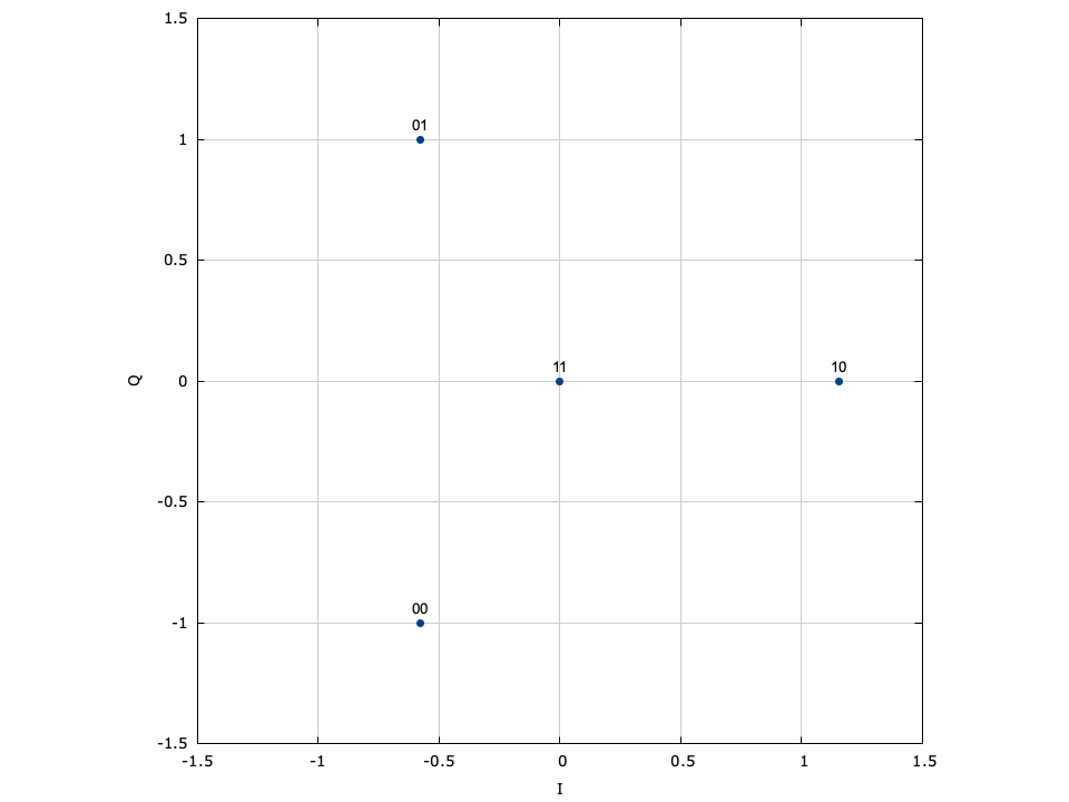
Figure [fig-modem-apsk-4]. 4-APSK (1,3)
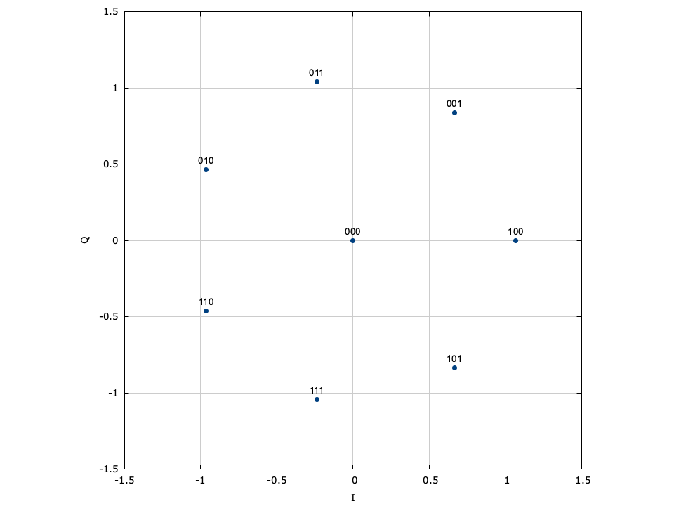
Figure [fig-modem-apsk-8]. 8-APSK (1,7)
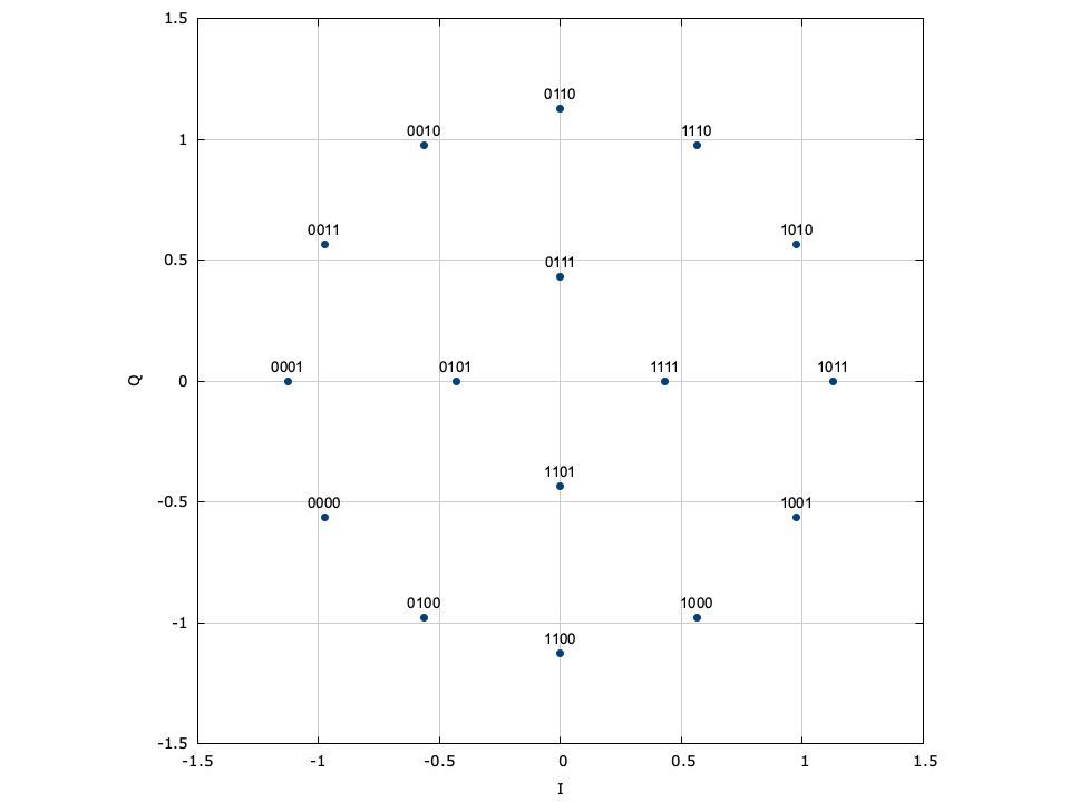
Figure [fig-modem-apsk-16]. 16-APSK (4,12)
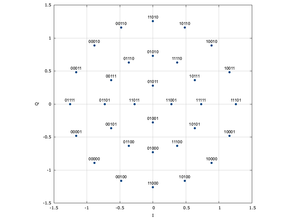
Figure [fig-modem-apsk-32]. 32-APSK (4,12,16)
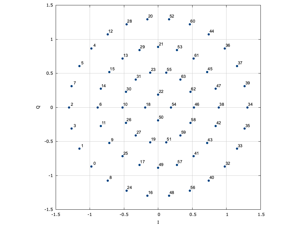
Figure [fig-modem-apsk-64]. 64-APSK (4,14,20,26)
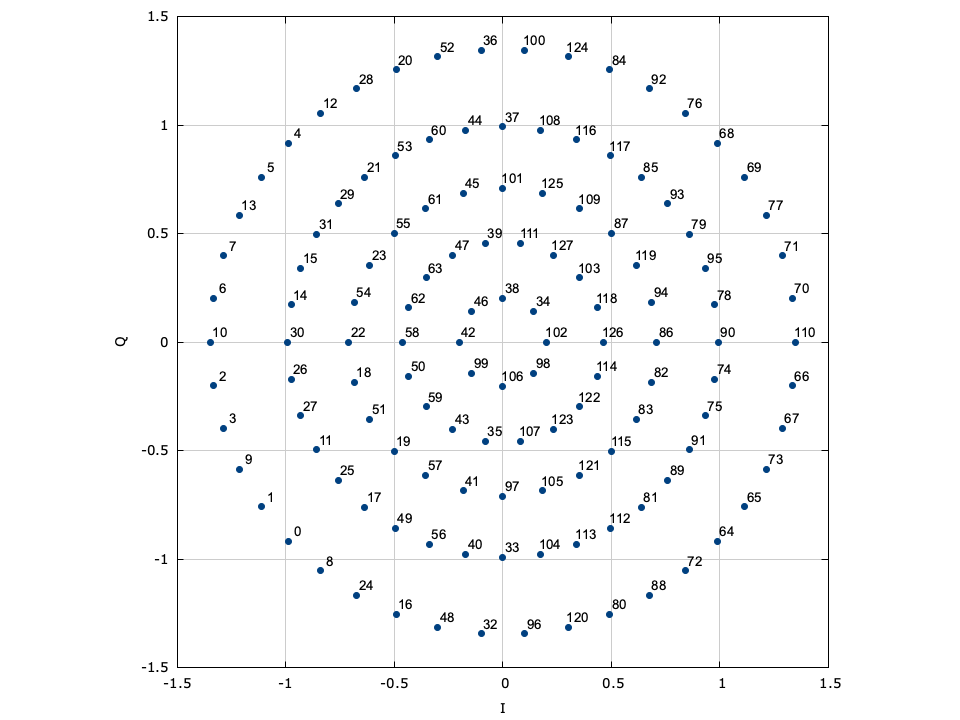
Figure [fig-modem-apsk-128]. 128-APSK (8,18,24,36,42)
Figure [fig-modem-apsk]. Amplitude/phase-shift keying (APSK) modem demonstrating constellation points lying on concentric circles. Not shown is 256-APSK (6,18,32,36,46,54,64).
[ref:fig-modem-apsk] depicts the available APSK signal constellations for \(M\) up to 128. The constellation points and bit mappings have been optimized to minimize the bit error rate in 10 dB SNR.
LIQUID_MODEM_ASK (amplitude-shift keying)∞
Amplitude-shift keying (ASK) is a simple form of amplitude modulation by which the information is encoded entirely in the in-phase component of the baseband signal. The encoded symbol is simply
$$ s_k = \alpha \bigl( 2 k - M - 1 \bigr) $$where \(\alpha\) is a scaling factor to ensure \(E\{s_k^2\}=1\) ,
$$ \alpha = \begin{cases} 1 & M=2 \\ 1/\sqrt{5} & M=4 \\ 1/\sqrt{21} & M=8 \\ 1/\sqrt{85} & M=16 \\ 1/\sqrt{341} & M=32 \\ \sqrt{3}/M & M \gt 32 \end{cases} $$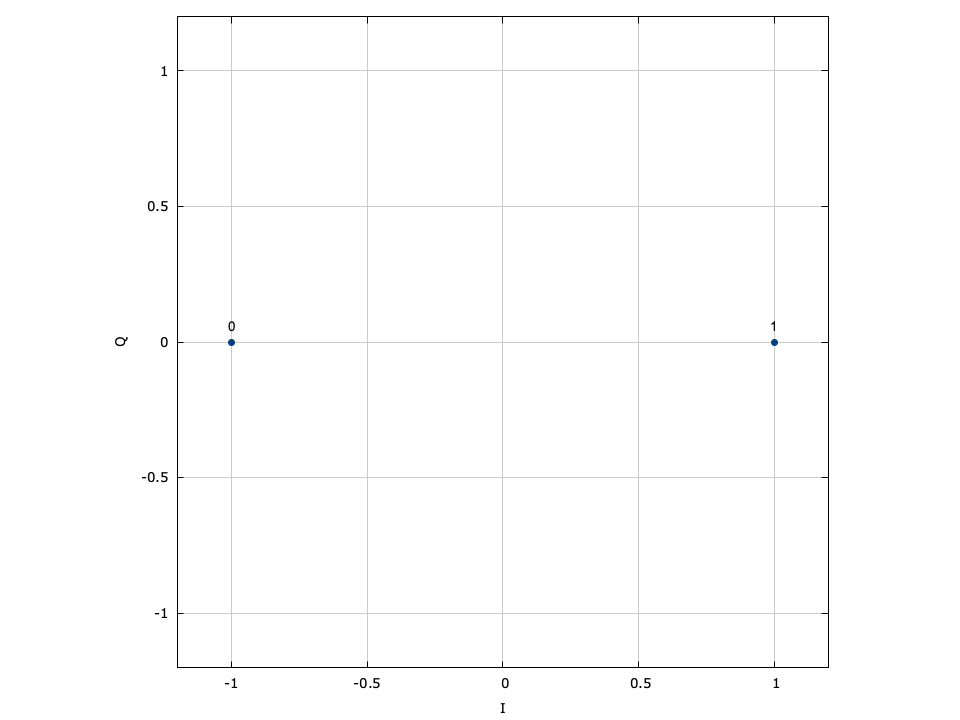
Figure [fig-modem-ask-2]. 2-ASK
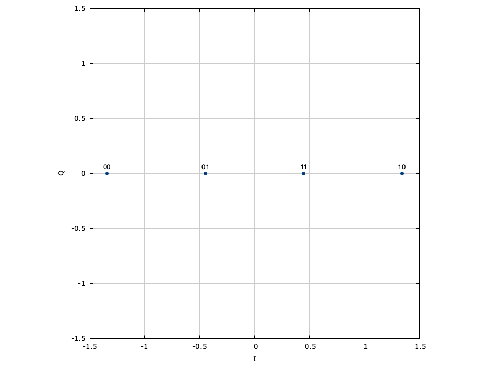
Figure [fig-modem-ask-4]. 4-ASK
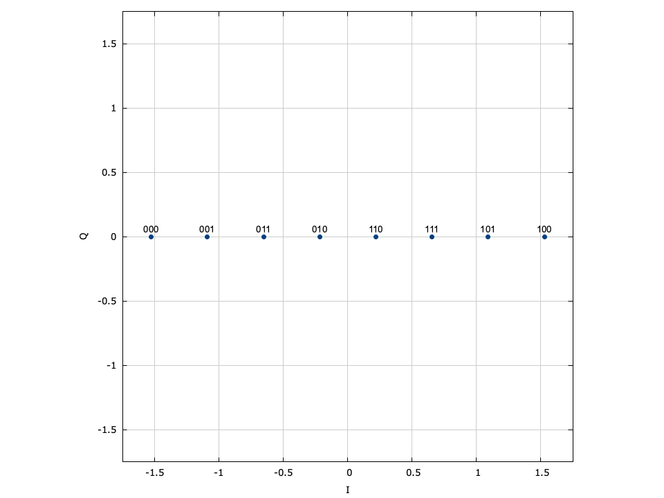
Figure [fig-modem-ask-8]. 8-ASK
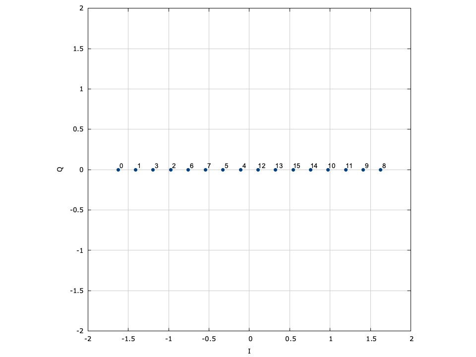
Figure [fig-modem-ask-16]. 16-ASK
Figure [fig-modem-ask]. Pulse-amplitude modulation (ASK) modem}
[ref:fig-modem-ask] depicts the ASK constellation map for \(M\) up to 16. Due to the poor error rate performance of ASK values of \(M\) greater than 16 are not recommended.
LIQUID_MODEM_QAM (quadrature amplitude modulation)∞
Also known as quadrature amplitude-shift keying, QAM modems encode data using both the in-phase and quadrature components of a signal amplitude. In fact, the symbol is split into independent in-phase and quadrature symbols which are encoded separately as LIQUID_MODEM_ASK symbols. Gray encoding is applied to both the I and Q symbols separately to help ensure minimal bit changes between adjacent samples across both in-phase and quadrature-phase dimensions. This is made evident in [ref:fig-modem-qam-64] where one can see that the first three bits of the symbol encode the in-phase component of the sample, and the last three bits encode the quadrature component of the sample. We may formally describe the encoded sample is
$$ s_k = \alpha \Bigl\{ ( 2 k_i - M_i - 1 ) + j(2 k_q - M_q - 1) \Bigr\} $$where\(k_i\) is the in-phase symbol,\(k_q\) is the quadrature symbol,\(M_i = 2^{m_i}\) and \(M_q = 2^{m_q}\) , are the number of respective in-phase and quadrature symbols,\(m_i=\lceil \log_2(M) \rceil\) and \(m_q=\lfloor \log_2(M) \rfloor\) are the number of respective in-phase and quadrature bits, and\(\alpha\) is a scaling factor to ensure \(E\{s_k^2\}=1\) ,
$$ \alpha = \begin{cases} 1/\sqrt{2} & M=4 \\ 1/\sqrt{6} & M=8 \\ 1/\sqrt{10} & M=16 \\ 1/\sqrt{26} & M=32 \\ 1/\sqrt{42} & M=64 \\ 1/\sqrt{106} & M=128 \\ 1/\sqrt{170} & M=256 \\ 1/\sqrt{426} & M=512 \\ 1/\sqrt{682} & M=1024 \\ 1/\sqrt{1706} & M=2048 \\ 1/\sqrt{2730} & M=4096 \\ \sqrt{2/M} & \text{else} \end{cases} $$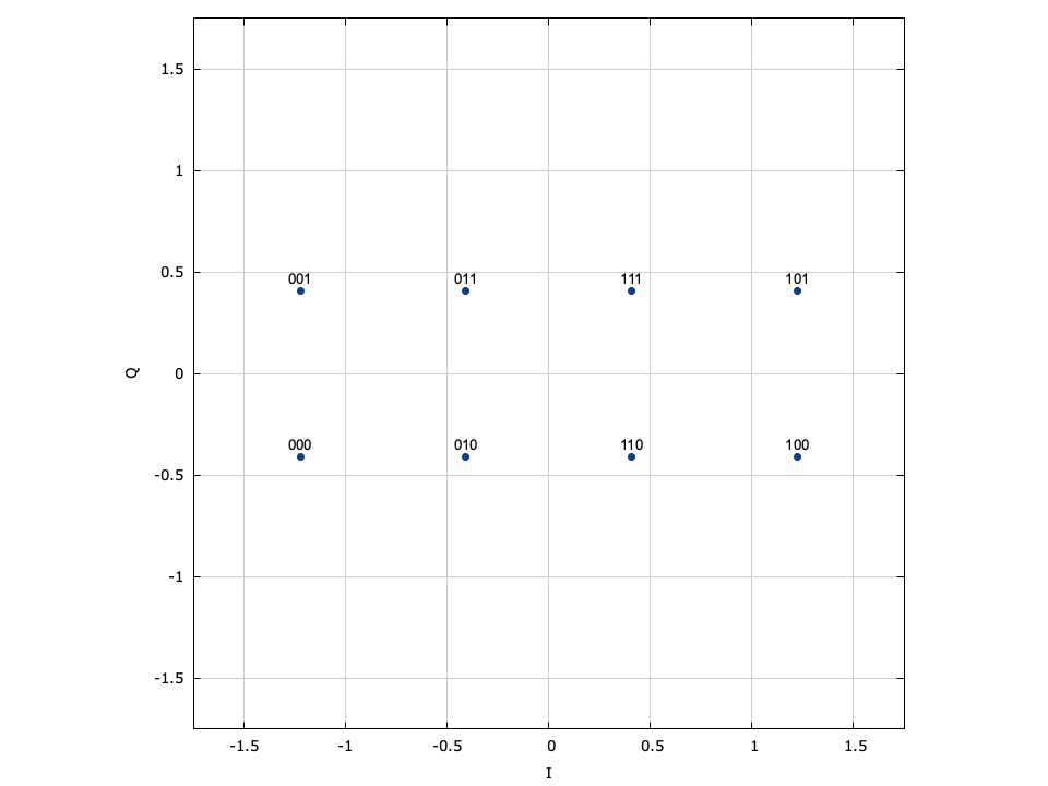
Figure [fig-modem-qam-8]. 8-QAM
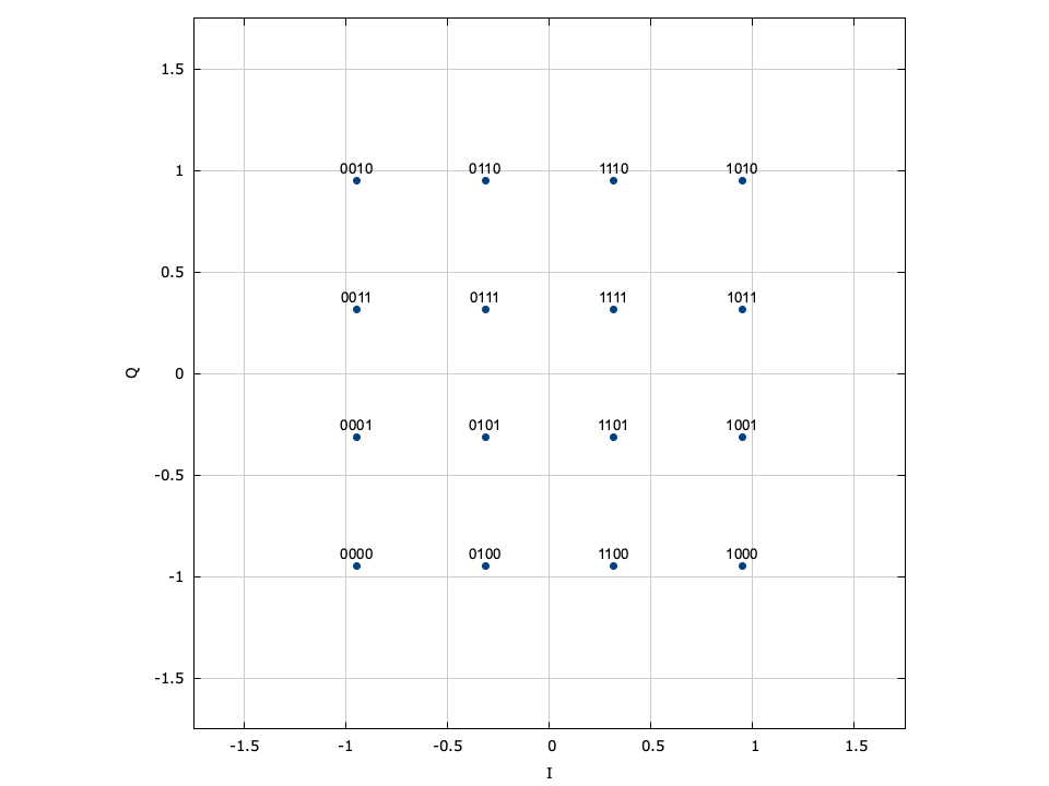
Figure [fig-modem-qam-16]. 16-QAM
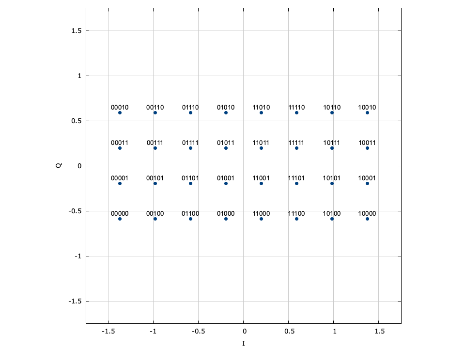
Figure [fig-modem-qam-32]. 32-QAM
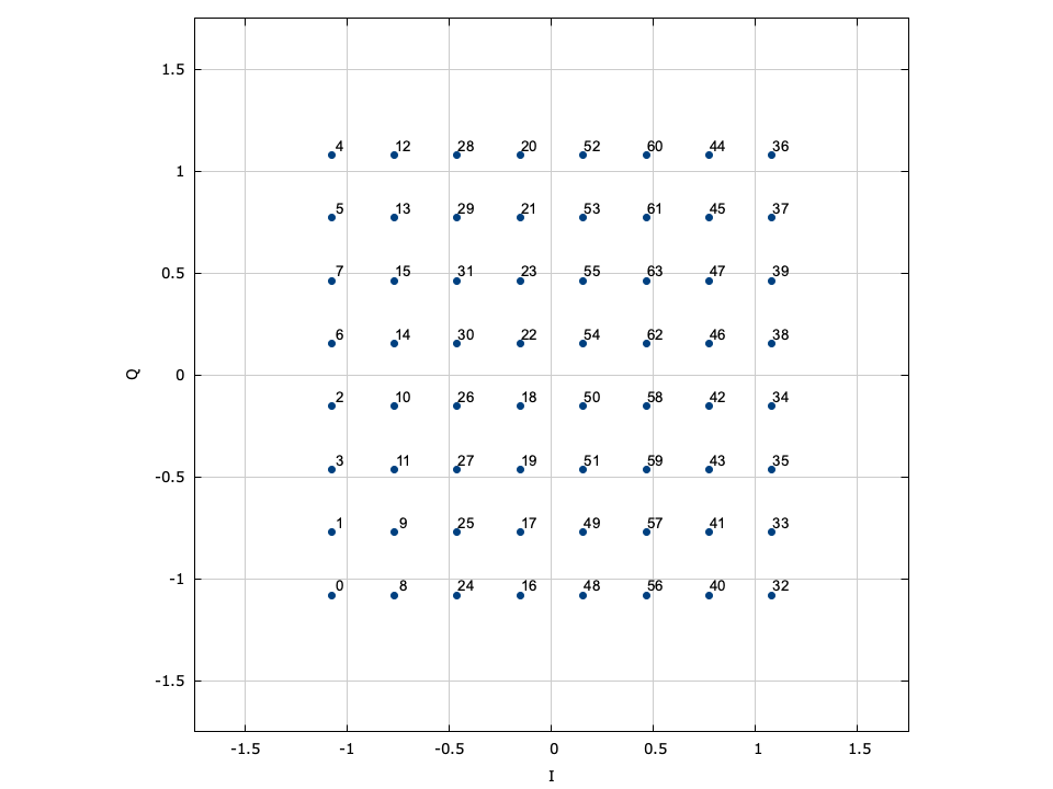
Figure [fig-modem-qam-64]. 64-QAM
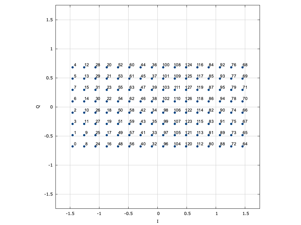
Figure [fig-modem-qam-128]. 128-QAM
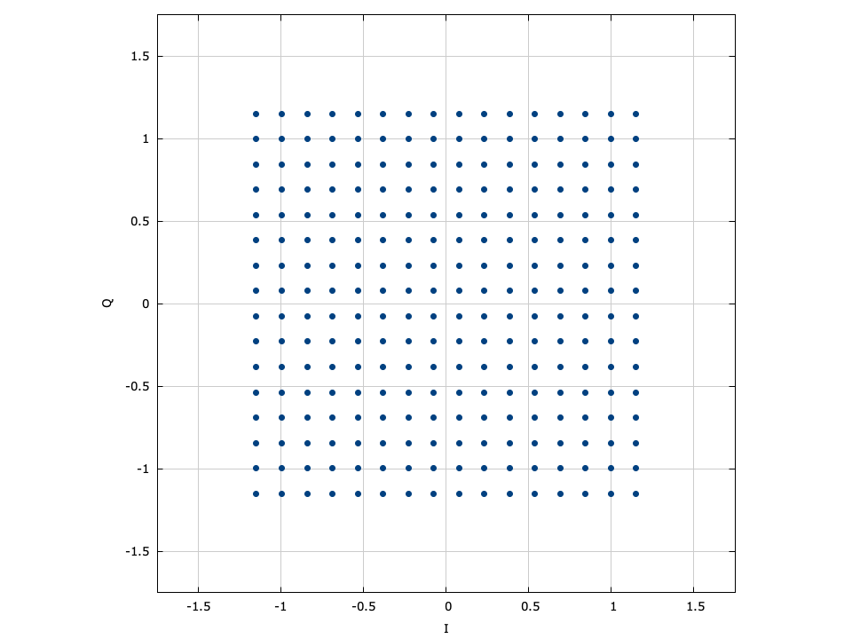
Figure [fig-modem-qam-256]. 256-QAM
Figure [fig-modem-qam]. Rectangular quaternary-amplitude modulation (QAM) modem
[ref:fig-modem-qam] depicts the arbitrary rectangular QAM modem constellation maps for \(M\) up to 256. Notice that all the symbol points are gray encoded to minimize bit errors between adjacent symbols.
LIQUID_MODEM_ARB (arbitrary modem)∞
liquid also allows the user to create their own modulation schemes by designating the full signal constellation. The penalty for defining a constellation as an arbitrary set of points is that it cannot be decoded systematically. All of the previous modulation schemes have the benefit of being very fast to decode, and do not necessitate searching over the entire constellation space to find the nearest symbol. An example interface for generating a pair of arbitrary modems is listed below.
#include <liquid/liquid.h>

int main() {
    // set modulation depth (bits/symbol)
    unsigned int bps=4;
    float complex constellation[1<<bps];

    // ... (initialize constellation) ...

    // create the arbitrary modem objects
    modem mod   = modem_create_arbitrary(constellation, 1<<bps);
    modem demod = modem_create_arbitrary(constellation, 1<<bps);

    // ... (modulate and demodulate as before) ...

    // destroy modem objects
    modem_destroy(mod);
    modem_destroy(demod);
}
Several pre-defined arbitrary signal constellations are available, including optimal QAM constellations, and some other fun (but perhaps not so useful) modulation schemes.
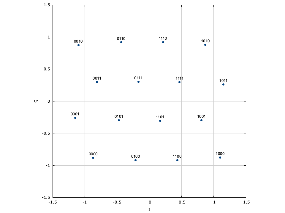
Figure [fig-modem-optqam-16opt]. optimal 16-QAM
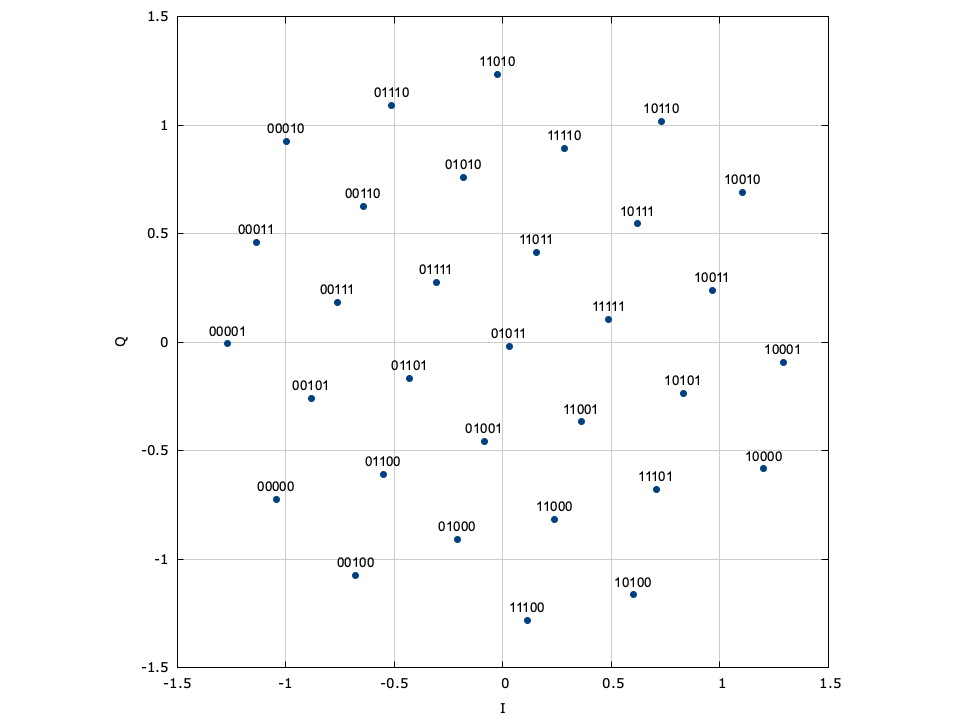
Figure [fig-modem-optqam-32opt]. optimal 32-QAM
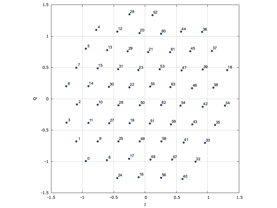
Figure [fig-modem-optqam-64opt]. optimal 64-QAM
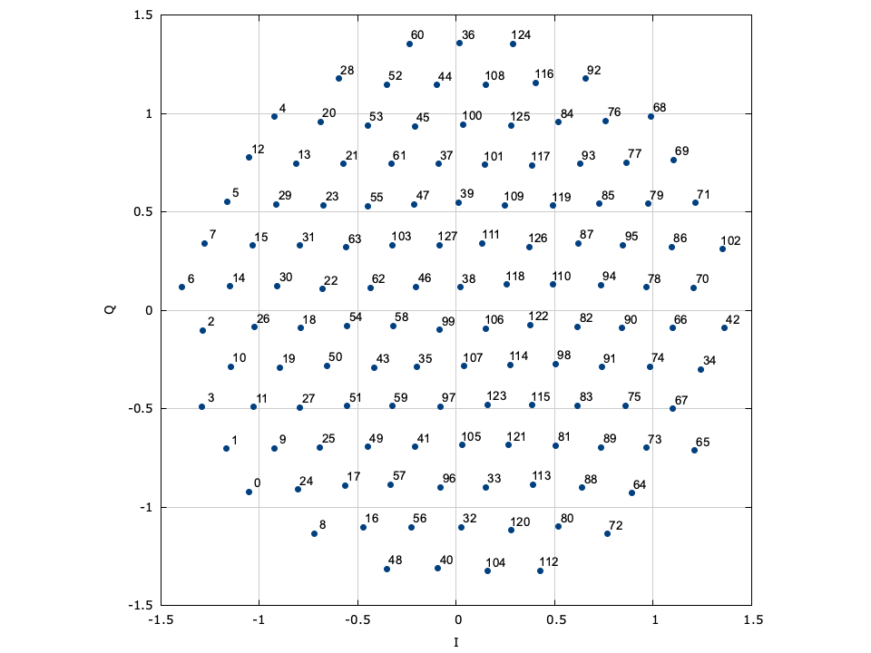
Figure [fig-modem-optqam-128opt]. optimal 128-QAM
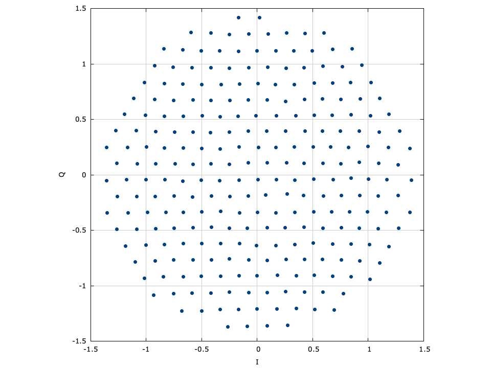
Figure [fig-modem-optqam-256opt]. optimal 256-QAM
Figure [fig-modem-optqam]. Optimal \(M\) -QAM constellation maps.
[ref:fig-modem-optqam] shows the constellation maps for the optimal QAM schemes. Notice that the constellations approximate a circle with each point falling on the lattice of equilateral triangles. Furthermore, adjacent constellation points differ by typically only a single bit to reduce the resulting bit error rate at the output of the demodulator. These constellations marginally out-perform regular square QAM (see Figures [ref:fig-modem-M32] and [ref:fig-modem-M128] ) at the expense of a significantly increased computational complexity.
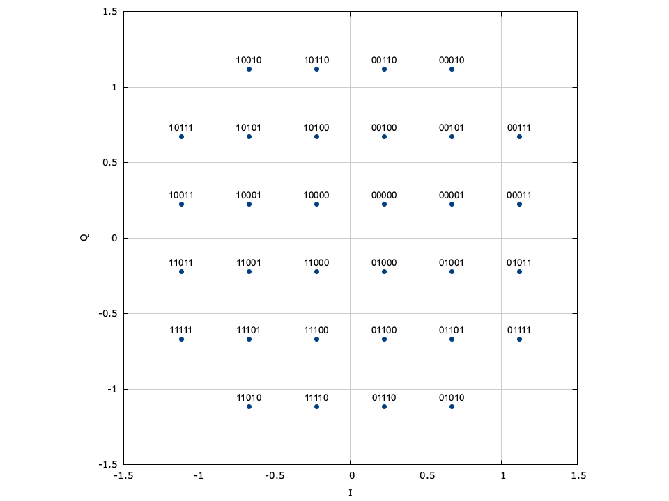
Figure [fig-modem-arb-sqam32]. "square" 32-QAM
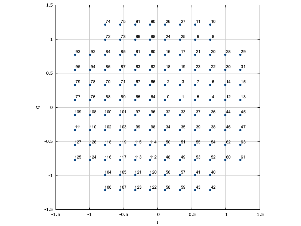
Figure [fig-modem-arb-sqam128]. "square" 128-QAM
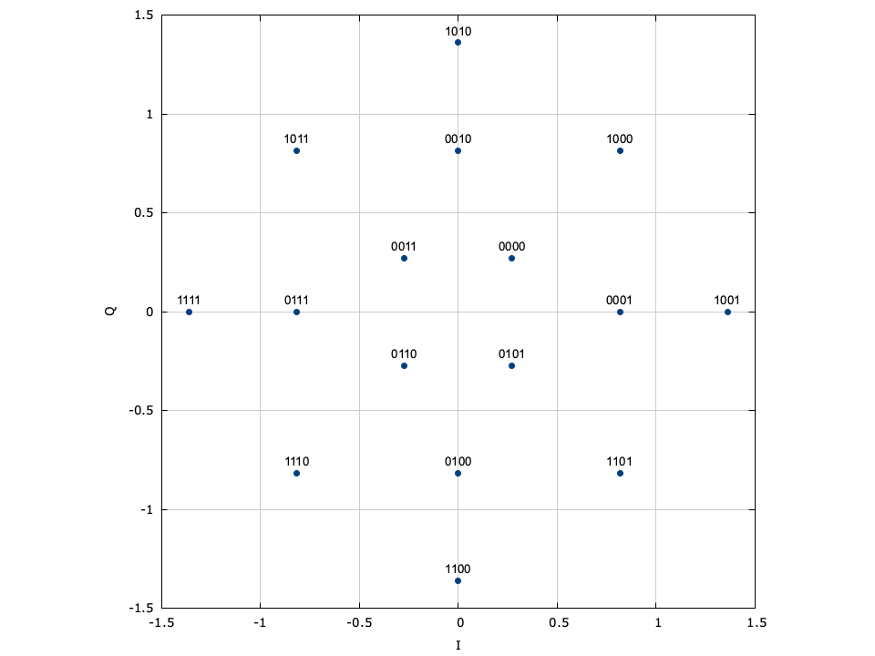
Figure [fig-modem-arb-V29]. V.29
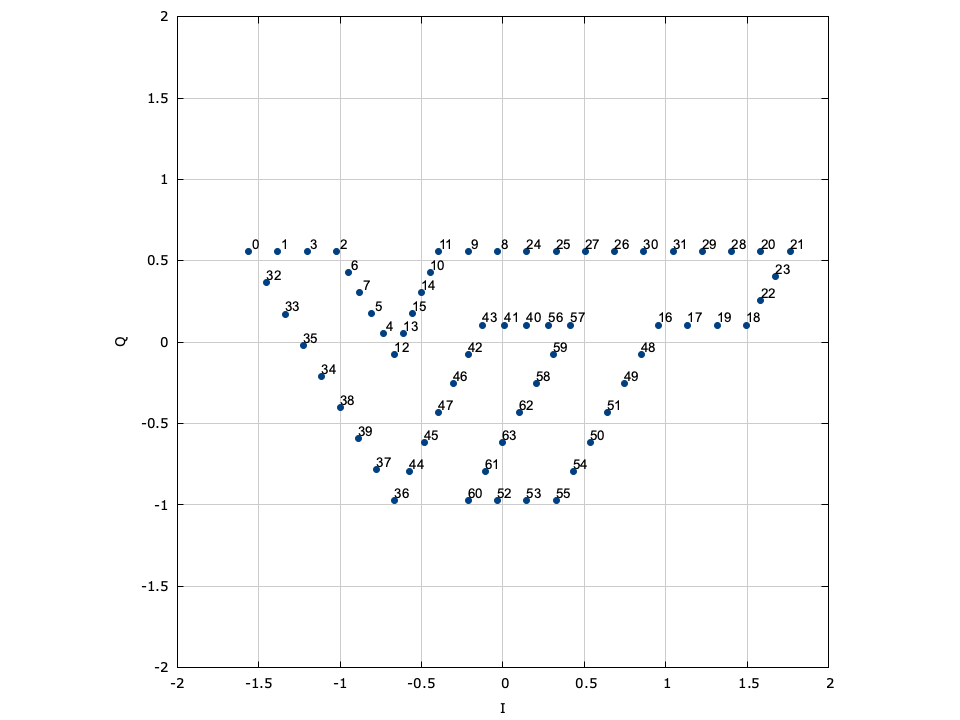
Figure [fig-modem-arb-64vt]. 64-VT
Figure [fig-modem-arb]. Arbitrary constellation (ARB) modem
[ref:fig-modem-arb] depicts several available arbitrary constellation maps; however the user can create any arbitrary constellation map so long as no two points overlap (see modem_arb_init() and modem_arb_init_file() in[ref:section-modem-digital-interface] ).
Performance∞
As discussed in [ref:section-fec-performance] , the performance of an error-correction scheme is typically measured in the bit error rate (BER)|the average error probability for a bit to be in error in the presence of additive white Gauss noise (AWGN).
.. footnote
assuming the modulated symbols are uncorrelated and
identically distributed.
The bit error rate (BER) performance of the different available modulation schemes can be seen in Figures [ref:fig-modem-M2] --[ref:ref-fig-modem-M256] , relative to the ratio of energy per bit to noise power (\(E_b/N_0\) ). The raw data can be found in the doc/data/modem-ber/ subdirectory.
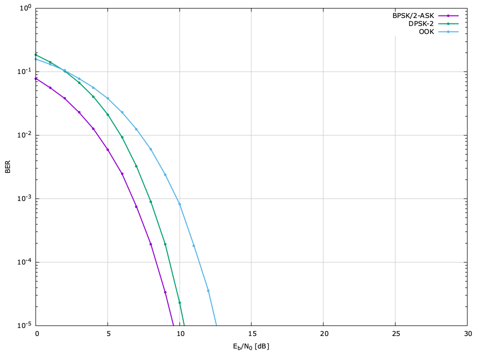
Figure [fig-modem-M2]. Bit error rates vs. \(E_b/N_0\) for \(M=2\) .
\(M=2\) BER performance, \(\hat{P}=10^{-5}\)
| Scheme | \(E_s/N_0\) | \(E_b/N_0\) |
| BPSK, 2-ASK | 9.59 | 9.59 |
| DBPSK | 10.46 | 10.46 |
| OOK | 12.61 | 12.61 |
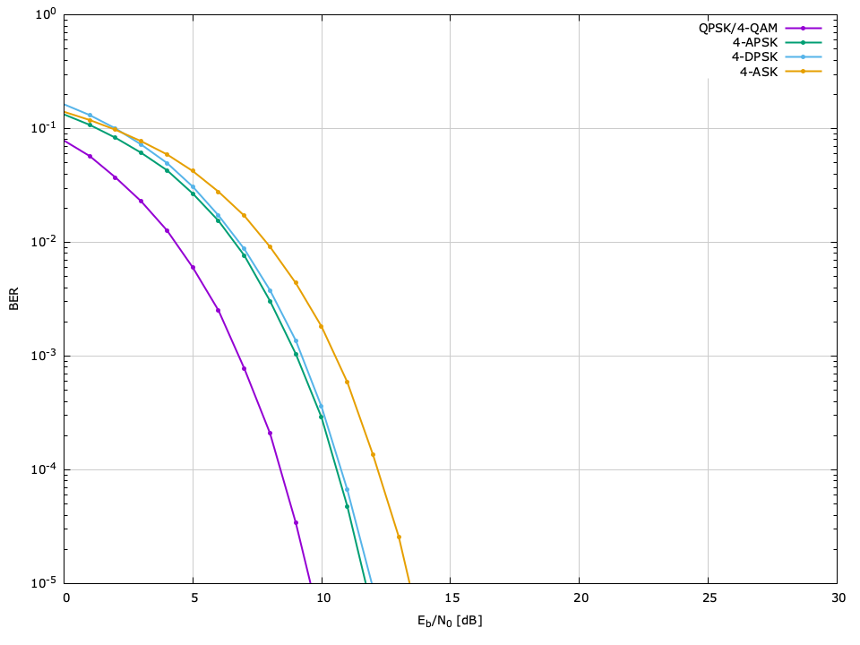
Figure [fig-modem-M4]. Bit error rates vs. \(E_b/N_0\) for \(M=4\) .
\(M=4\) BER performance, \(\hat{P}=10^{-5}\)
| Scheme | \(E_s/N_0\) | \(E_b/N_0\) |
| QPSK, 4-QAM | 12.59 | 9.59 |
| 4-APSK | 14.76 | 11.75 |
| DQPSK | 14.93 | 11.92 |
| 4-ASK | 16.59 | 13.58 |

Figure [fig-modem-M8]. Bit error rates vs. \(E_b/N_0\) for \(M=8\) .
\(M=8\) BER performance, \(\hat{P}=10^{-5}\)
| Scheme | \(E_s/N_0\) | \(E_b/N_0\) |
| 8-APSK | 16.12 | 11.35 |
| 8-QAM | 17.28 | 12.51 |
| 8-PSK | 17.84 | 13.07 |
| 8-DPSK | 20.62 | 15.85 |
| 8-ASK | 22.61 | 17.84 |
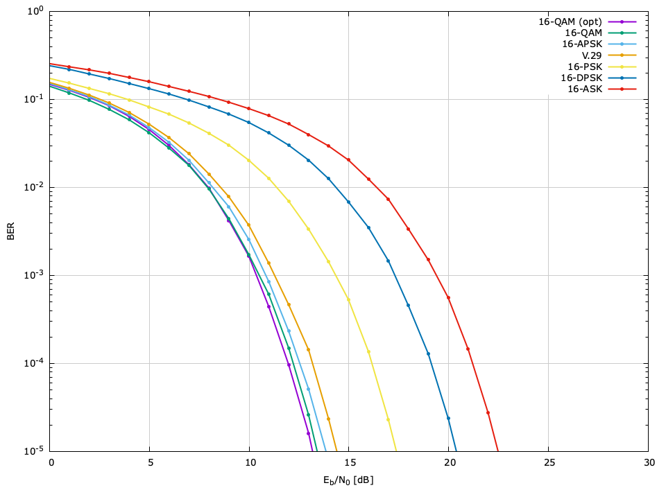
Figure [fig-modem-M16]. Bit error rates vs. \(E_b/N_0\) for \(M=16\) .
\(M=16\) BER performance, \(\hat{P}=10^{-5}\)
| Scheme | \(E_s/N_0\) | \(E_b/N_0\) |
| ARB-16-OPT | 19.15 | 13.13 |
| 16-QAM | 19.57 | 13.55 |
| 16-APSK | 19.92 | 13.90 |
| V.29 | 20.48 | 14.45 |
| 16-PSK | 23.43 | 17.41 |
| 16-DPSK | 26.43 | 20.41 |
| 16-ASK | 28.54 | 22.52 |
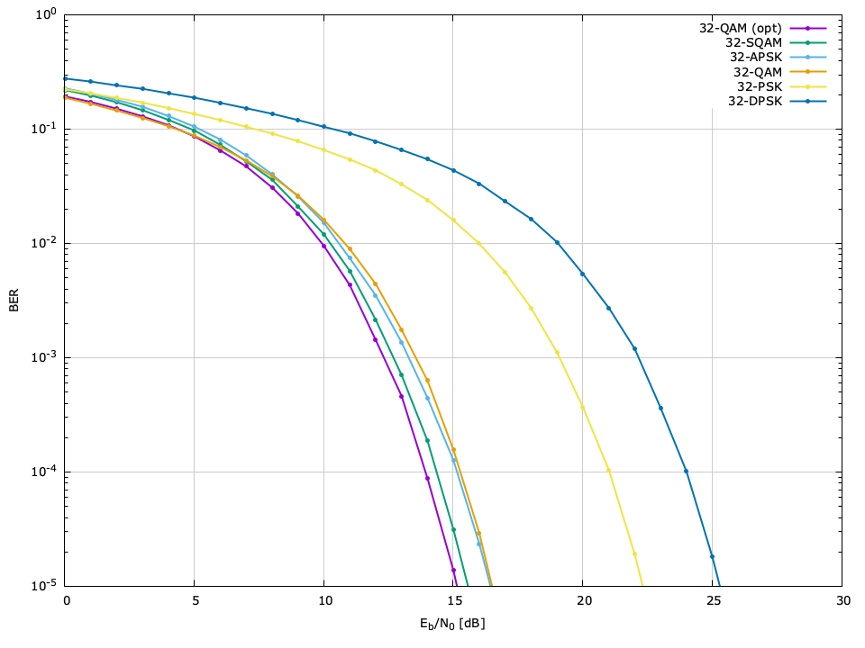
Figure [fig-modem-M32]. Bit error rates vs. \(E_b/N_0\) for \(M=32\) .
\(M=32\) BER performance, \(\hat{P}=10^{-5}\)
| Scheme | \(E_s/N_0\) | \(E_b/N_0\) |
| ARB-32-OPT | 22.11 | 15.12 |
| 32-SQAM | 22.56 | 15.57 |
| 32-APSK | 23.43 | 16.44 |
| 32-QAM | 23.59 | 16.60 |
| 32-PSK | 29.38 | 22.38 |
| 32-DPSK | 32.38 | 25.39 |
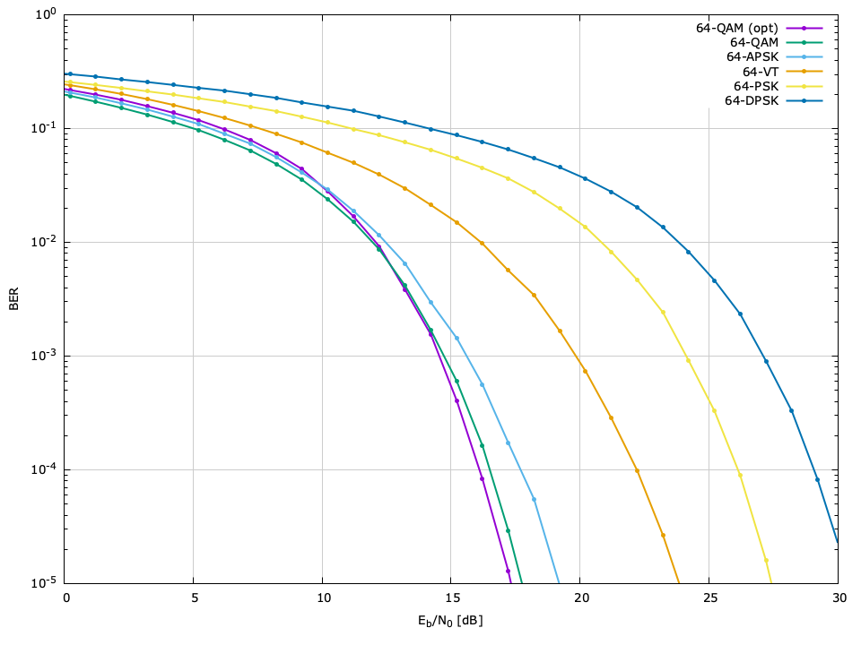
Figure [fig-modem-M64]. Bit error rates vs. \(E_b/N_0\) for \(M=64\) .}
\(M=64\) BER performance, \(\hat{P}=10^{-5}\)
| Scheme | \(E_s/N_0\) | \(E_b/N_0\) |
| ARB-64-OPT | 25.22 | 17.44 |
| 64-QAM | 25.50 | 17.71 |
| 64-APSK | 27.06 | 19.28 |
| ARB-64-VT | 31.67 | 23.89 |
| 64-PSK | 35.32 | 27.38 |
| 64-DPSK | 38.28 | 30.50 |
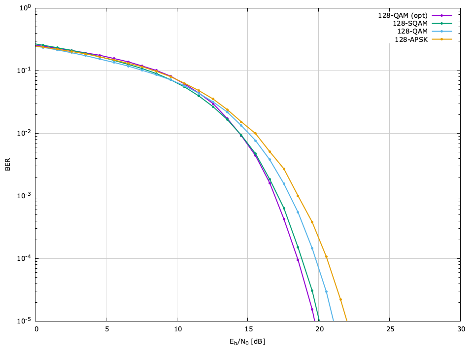
Figure [fig-modem-M128]. Bit error rates vs. \(E_b/N_0\) for \(M=128\) .}
\(M=128\) BER performance, \(\hat{P}=10^{-5}\)
| Scheme | \(E_s/N_0\) | \(E_b/N_0\) |
| ARB-128-OPT | 28.19 | 19.74 |
| 128-SQAM | 28.42 | 19.97 |
| 128-QAM | 29.60 | 21.15 |
| 128-APSK | 30.55 | 22.10 |
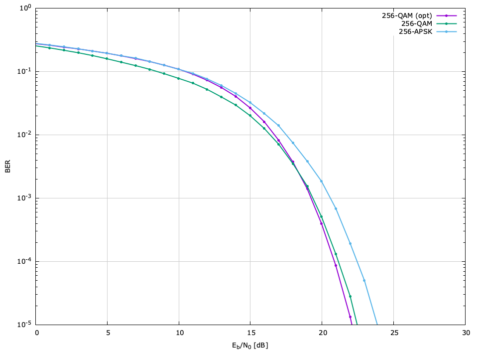
Figure [fig-modem-M256]. Bit error rates vs. \(E_b/N_0\) for \(M=256\) .
\(M=256\) BER performance, \(\hat{P}=10^{-5}\)
| Scheme | \(E_s/N_0\) | \(E_b/N_0\) |
| ARB-256-OPT | 31.09 | 22.06 |
| 256-QAM | 31.56 | 22.53 |
| 256-APSK | 33.10 | 24.06 |
Soft Demodulation∞
Unlike hard demodulation which seeks the most likely transmitted symbol for a given received sample, the goal of soft demodulation is to derive a probability metric for each bit for the received sample. When using the output of the demodulator in conjunction with forward error-correction coding, the soft bit information can improve the error detection and correction capabilities of most decoders, usually by about 1.5 dB. This soft bit information provides a clue to the decoder as to the confidence that each bit was received correctly. For turbo-product codes {cite:Berrou:1993} and low-density parity check (LDPC) codes {cite:Gallager:1962}, this soft bit information is nearly a requirement.
Before we continue, let us define some nomenclature:
- \(M=2^m\) are the number of points in the constellation (constellation size).
- \(m=\log_2(M)\) are the number of bits per symbol in the constellation (modulation depth).
- \(s_k\) is the symbol at index \(k\) on the complex plane;\(k \in \{0,1,2,\ldots,M-1\}\) .
- \(\{b_0,b_1,\ldots,b_{m-1}\}\) is the encoded bit string of \(s_k\) and is simply the value of \(k\) in binary-coded decimal.
- \(b_j\) is the bit at index \(j\) ;\(b_j \in \{0,1\}\) and \(j \in \{0,1,\ldots,m-1\}\) .
- \(\mathcal{S}_M = \{s_0,s_1,\ldots,s_{M-1}\}\) is the set of all symbols in the constellation where\(1/M \sum_k \|s_k\|_2^2 = 1\) .
- \(\mathcal{S}_{b_j=t}\) is the subset of \(\mathcal{S}_M\) where the bit at index \(j\) is equal to \(t \in \{0,1\}\) .
For example, let the modulation scheme be the generic 4-PSK with the constellation map defined in [ref:fig-modem-psk-4] which has \(m=2\) , \(M=4\) , and\(\mathcal{S}_M = \{s_0=1, s_1=j, s_2=-j, s_3=-1\}\) . Subsets:
- \(\mathcal{S}_{b_0=0} = \{s_0= 1, s_2=-j\}\) (right-most bit is 0 )
- \(\mathcal{S}_{b_0=1} = \{s_1= j, s_3=-1\}\) (right-most bit is 1 )
- \(\mathcal{S}_{b_1=0} = \{s_0= 1, s_1= j\}\) (left-most bit is 0 )
- \(\mathcal{S}_{b_1=1} = \{s_2=-j, s_3=-1\}\) (left-most bit is 1 )
A few key points:
- \(\mathcal{S}_{b_j=0} \cap \mathcal{S}_{b_j=1} = \emptyset, \, \forall_j\) .
- \(\mathcal{S}_{b_j=0} \cup \mathcal{S}_{b_j=1} = \mathcal{S}_M, \, \forall_j\) .
Let us represent the received signal at a sampling instant \(n\) as
$$ r(n) = s(n) + w(n) $$where \(s\) is the transmitted symbol and \(w\) is a zero-mean complex Gauss random variable with a variance \(\sigma_n^2 = E\{w w^*\}\) . Let the transmitted symbols be i.i.d. and drawn from a \(M\) -point constellation, each with \(m\) bits of information such that the symbols belong to a set of constellation points\(s_k \in \mathcal{S}_M\) and \(E\{s_k s_k^*\}=1\) . Assuming perfect channel knowledge, timing, and carrier offset recovery, the log-likelihood ratio (LLR) of each bit \(b_j\) is shown to be {cite:LeGoff:1994(Eq. (8))} the ratio of the two conditional a posteriori probabilities of each bit having been transmitted, viz.
$$ \Lambda(b_j) = \ln \frac{ P\left(b_j=1 | \text{observation} \right) }{ P\left(b_j=0 | \text{observation} \right) } $$Assuming that the channel is memoryless the "observation" is simply the received sample \(r\) in ([ref:eqn-modem-digital-soft-received_signal] ) and does not depend on previous symbols; therefore\(P\left(b_j=t|\text{observation}\right) = P\left(b_j=t|r(n)\right)\) and \(t \in \{0,1\}\) . Furthermore, by assuming that the transmitted symbols are equally probable and that the noise follows a Gauss distribution {cite:Qiang:2003} the LLR reduces to
$$ \Lambda(b_j) = \ln \Biggl( \sum_{s^+\in \mathcal{S}_{b_j=1}} { \exp\Bigl\{\|r-s^+\|_2^2 / 2 \sigma_n^2\Bigr\} } \Biggr) -\ln \Biggl( \sum_{s^-\in \mathcal{S}_{b_j=0}} { \exp\Bigl\{\|r-s^-\|_2^2 / 2 \sigma_n^2\Bigr\} } \Biggr) $$As shown in {cite:Qiang:2003} a sub-optimal simplified LLR expression can be obtained by replacing the summations in ([ref:eqn-modem-digital-soft-LLR] ) with the single largest component of each: \(\ln \sum_j {e^{z_j}} \approx \max_j \ln (e^{z_j}) = \max_j z_j\) . This approximation provides a tight bound as long as the sum is dominated by its largest component. The approximate LLR becomes
$$ \tilde{\Lambda}(b_j) = \frac{1}{2\sigma_n^2} \Bigl\{ \underset{s^+\in \mathcal{S}_{b_j=0}}{\min} \|r-s^+\|_2^2 - \underset{s^-\in \mathcal{S}_{b_j=1}}{\min} \|r-s^-\|_2^2 \Bigr\} $$Conveniently, both the exponential and logarithm operations disappear; furthermore, the noise variance becomes a scaling factor and is only used to influence the reliability of the obtained LLR.
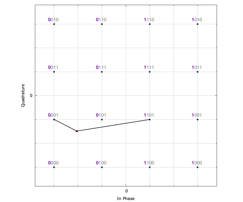
Figure [fig-modem-demodsoft-b0]. \(\tilde{\Lambda}(b_0) = -10.55\)
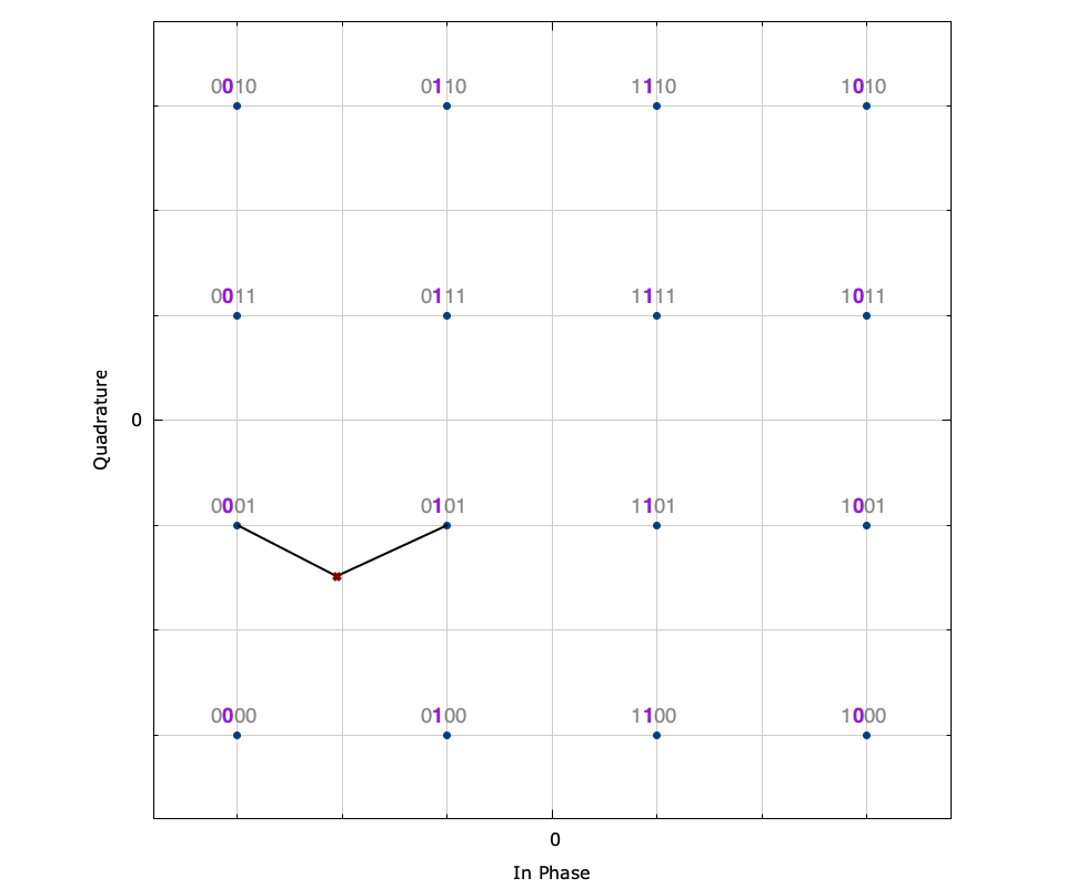
Figure [fig-modem-demodsoft-b1]. \(\tilde{\Lambda}(b_1) = -0.28\)
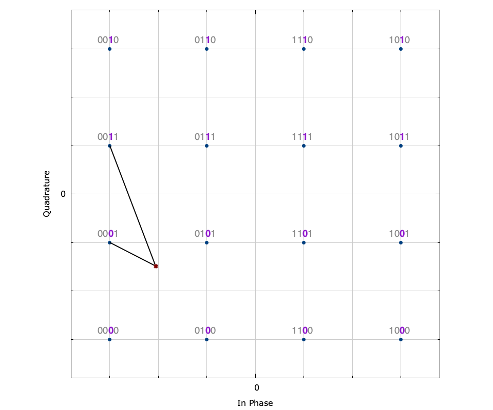
Figure [fig-modem-demodsoft-b2]. \(\tilde{\Lambda}(b_2) = -7.43\)
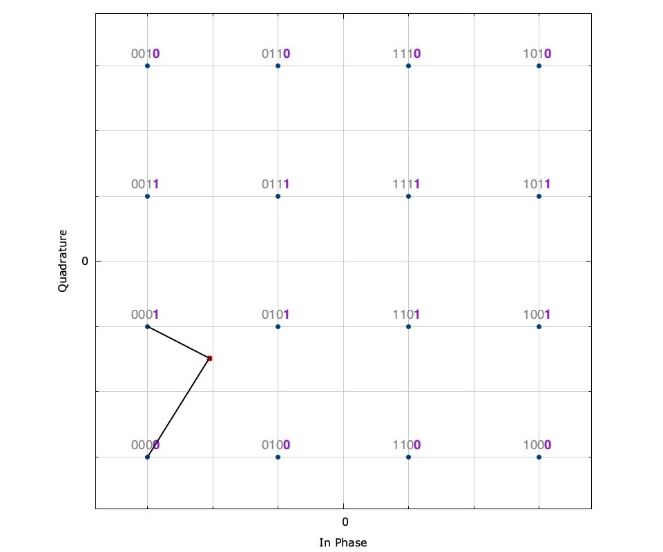
Figure [fig-modem-demodsoft-b3]. \(\tilde{\Lambda}(b_3) = 2.57\)
Figure [fig-modem-demodsoft]. Soft demodulation example of a 16-QAM sample. Each plot depicts the soft demodulation of each of the 4 bits where the \(\times\) denotes the received sample and the lines connect it to the nearest symbol with each of a 0 and 1 bit. The noise standard deviation is \(\sigma_n=0.2\) .
[ref:fig-modem-demodsoft] depicts the soft bit demodulation algorithm for a received 16-QAM signal point, corrupted by noise. The received sample is \(r = -0.65 - j0.47\) which results in a hard demodulation of 0001 . The subfigures depict each of the four bits in the symbol\(\{b_0,b_1,b_2,b_3\}\) for which the soft bit output is given, and show the nearest symbol for which a 0 and a 1 at that particular bit index occurs. For example, [ref:fig-modem-demodsoft-b2] shows that the nearest symbol containing a 0 at bit index 2 is \(s_1=\) 0001 (the hard decision demodulation) at \((-3 - j)/\sqrt{10}\) while the nearest symbol containing a 1 at bit index 2 is \(s_3=\) 0011 at \((-3 + j)/\sqrt{10}\) . Plugging \(s^-=s_1\) and \(s^+=s_3\) into ([ref:eqn-modem-digital-soft-LLR_approx] ) and evaluating for \(\sigma_n=0.2\) gives\(\tilde{\Lambda}(b_2) = -7.43\) . Because this number is largely negative, it is very likely that the transmitted bit \(b_2\) was 0 . This can be verified by [ref:fig-modem-demodsoft-b2] which shows that the distance from \(r\) to \(s^-\) is much shorter than that of \(s^+\) .
Conversely, [ref:fig-modem-demodsoft-b1] shows that \(b_1\) cannot be demodulated with such certainty; the distances from \(r\) to each of \(s^+\) and \(s^-\) are about the same. This is reflected in the relatively small LLR value of\(\tilde{\Lambda}(b_1)=-0.28\) which suggests a high uncertainty in the demodulation of \(b_1\) .
One major drawback of computing ([ref:eqn-modem-digital-soft-LLR_approx] ) is that finding the maximum requires searching over all constellation points to find the one which minimizes \(\|r-s_k\|\) (where \(s_k \in \mathcal{S}_{b_j=t}\) ) is particularly time-consuming. To circumvent this, liquid only searches over a subset\(\mathcal{S}_k \subset \mathcal{S}_M\) nearest to the hard-demodulated symbol (\(\mathcal{S}_k\) will typically only have about four values). This can be done quickly because the hard-demodulated symbol can be found systematically for most modulation schemes (e.g. for LIQUID_MODEM_QAM only \(\mathcal{O}(\log_2 M)\) comparisons are needed to make a hard decision). If no symbols are found within \(\mathcal{S}_k\) for a given bit value such that \(\mathcal{S}_k \cap \mathcal{S}_{b_j=t} = \emptyset\) then the magnitude of \(\Lambda(b_j)\) is sufficiently large and contains little soft bit information; that is\(\tilde{\Lambda}(b_j) \gg 0\) when \(\mathcal{S}_k \cap \mathcal{S}_{b_j=0} = \emptyset\) and\(\tilde{\Lambda}(b_j) \ll 0\) when \(\mathcal{S}_k \cap \mathcal{S}_{b_j=1} = \emptyset\) . It is guaranteed that\(\left( \mathcal{S}_k \cap \mathcal{S}_{b_j=0}\right) \cup \left( \mathcal{S}_k \cap \mathcal{S}_{b_j=1}\right) \neq \emptyset \) because \(s_k\) must be in either \(\mathcal{S}_{b_j=0}\) or\(\mathcal{S}_{b_j=1}\) .
liquid performs soft demodulation with the modem_demodulate_soft(q,x,*symbol,*soft_bits) method. This is the same as the regular demodulate method, but also returns the "soft" bits in addition to an estimate of the original symbol. Soft bit information is stored in liquid as type unsigned char with a value of 255 representing a "very likely 1 ", and a value of 0 representing a "very likely 0 ". The erasure condition is 127 .
Soft bit demodulation for soft-decision decoding
| Soft bit value | Interpretation |
| 0 | Very likely 0 |
| \(\vdots\) | \(\vdots\) |
| 63 | Likely 0 |
| \(\vdots\) | \(\vdots\) |
| 127 | Erasure |
| \(\vdots\) | \(\vdots\) |
| 191 | Likely 1 |
| \(\vdots\) | \(\vdots\) |
| 255 | Very likely 1 |
The fec and packetizer objects can make use of this soft information to improve the probability of decoding a packet (see [ref:section-fec-soft] and [ref:section-framing-packetizer] for details).
Error Vector Magnitude∞
The error vector magnitude (EVM) of a demodulated symbol is simply the average magnitude of the error vector between the received sample before demodulation and the expected transmitted symbol, viz.
$$ \textup{EVM} \triangleq \left| s - \hat{s} \right| $$EVM is returned by many of the framing objects (see [ref:section-framing] ) because it gives a good indication of signal distortion as a result of noise, inter-symbol interference, etc. If the only channel impairment is noise (e.g. perfect symbol timing) then the SNR can be estimated as
$$ \hat{\gamma} = E\left\{ \left| s - \hat{s} \right|^2 \right\}^{-1/2} $$