Gradient Search (gradsearch)
Keywords: gradsearch gradient descent search optimization
This module implements a gradient or "steepest-descent" search. Given a function \(f\) which operates on a vector\(\vec{x} = [x_0,x_1,\ldots,x_{N-1}]^T\) of \(N\) parameters, the gradient search method seeks to find the optimum \(\vec{x}\) which minimizes \(f(\vec{x})\) .
Theory∞
The gradient search is an iterative method and adjusts \(\vec{x}\) proportional to the negative of the gradient of \(f\) evaluated at the current location. The vector \(\vec{x}\) is adjusted by
$$ \Delta \vec{x}[n+1] = -\gamma[n] \nabla f(\vec{x}[n]) $$where \(\gamma[n]\) is the step size and\(\nabla f(\vec{x}[n])\) is the gradient of \(f\) at \(\vec{x}\) , at the \(n^{th}\) iteration. The gradient is a vector field which points to the greatest rate of increase, and is computed at \(\vec{x}\) as
$$ \nabla f(\vec{x}) = \left( \frac{\partial f}{\partial x_0}, \frac{\partial f}{\partial x_1}, \ldots, \frac{\partial f}{\partial x_{N-1}} \right) $$In most non-linear optimization problems, \(\nabla f(\vec{x})\) is not known, and must be approximated for each value of \(\vec{x}[n]\) using the finite element method. The partial derivative of the \(k^{th}\) component is estimated by computing the slope of \(f\) when \(x_k\) is increased by a small amount \(\Delta\) while holding all other elements of \(\vec{x}\) constant. This process is repeated for all elements in \(\vec{x}\) to compute the gradient vector. Mathematically, the \(k^{th}\) component of the gradient is approximated by
$$ \frac{\partial f(\vec{x})}{\partial x_k} \approx \frac{f(x_0,\ldots,x_k+\Delta,\ldots,x_{N-1}) - f(\vec{x})}{\Delta} $$Once \(\nabla f(\vec{x}[n])\) is known, \(\Delta\vec{x}[n+1]\) is computed and the optimizing vector is updated via
$$ \vec{x}[n+1] = \vec{x}[n] + \Delta\vec{x}[n+1] $$Momentum constant∞
When \(f(\vec{x})\) is flat (i.e. \(\nabla f(\vec{x})\approx \vec{0}\) ), convergence will be slow. This effect can be mitigated by permitting the update vector equation to retain a small portion of the previous step vector. The updated vector at time \(n+1\) is
$$ \vec{x}[n+1] = \vec{x}[n] + \Delta\vec{x}[n+1] + \alpha\Delta\vec{x}[n] $$where \(\Delta\vec{x}[0] = \vec{0}\) . The effective update at time \(n+1\) is
$$ \vec{x}[n+1] = \sum_{k=0}^{n+1}{\alpha^{k}\Delta\vec{x}[n+1-k]} $$which is stable only for \(0 \le \alpha \lt 1\) . For flat regions, the gradient vector \(\nabla f(\vec{x})\) is approximately a constant \(\Delta\vec{x}\) , and \(\vec{x}[n]\) therefore becomes a geometric series converging to \(\Delta\vec{x}/(1-\alpha)\) . This accelerates the algorithm across relatively flat regions of \(f\) . The momentum constant additionally adds some stability for regions where the gradient method tends to oscillate, such as steep valleys in \(f\) .
Step size adjustment∞
In liquid , the gradient is normalized to unity (orthonormal). That is \(\|\nabla f(\vec{x}[n])\|=1\) . Furthermore, \(\gamma\) is slightly reduced each epoch by a multiplier \(\mu\)
$$ \gamma[n+1] = \mu \gamma[n] $$This helps improve stability and convergence over regions where the algorithm might oscillate due to steep values of \(f\) .
Interface∞
Here is a summary of the parameters used in the gradient search algorithm and their default values:
- \(\Delta\) : step size in computing the gradient (default \(10^{-6}\) )
- \(\gamma\) : step size in updating \(\vec{x}[n]\) (default 0.002)
- \(\alpha\) : momentum constant (default 0.1)
- \(\mu\)
Here is the basic interface to the gradsearch object:
- gradsearch_create(*userdata,*v,n,utility,min/max,*props) creates a gradient search object designed to optimize an \(n\) -point vector \(\vec{v}\) . The user-defined utility function and userdata structures define the search, as well as the min/max flag which can be either LIQUID_OPTIM_MINIMIZE or LIQUID_OPTIM_MAXIMIZE . Finally, the search is parametrized by the props structure; if set to NULL the defaults will be used. When run the gradsearch object will update the "optimal" value in the input vector \(\vec{v}\) specified during create() .
- gradsearch_destroy(q) destroys a gradsearch object, freeing all internally-allocated memory.
- gradsearch_print(q) prints the internal state of the gradient search object.
- gradsearch_reset(q) resets the internal state of the gradient search object.
- gradsearch_step(q) steps through a single iteration of the gradient search. The result is stored in the original input vector \(\vec{v}\) specified during the create() method.
- gradsearch_execute(q,n,target_utility) runs multiple iterations of the search algorithm, stopping after either \(n\) iterations or if the target utility is met.
Here is an example of how the gradient_search is used:
#include <liquid/liquid.h>

// user-defined utility callback function
float myutility(void * _userdata, float * _v, unsigned int _n)
{
    float u = 0.0f;
    unsigned int i;
    for (i=0; i<_n; i++)
        u += _v[i] * _v[i];
    return u;
}

int main() {
    unsigned int num_parameters = 8;    // search dimensionality
    unsigned int num_iterations = 100;  // number of iterations to run
    float target_utility = 0.01f;       // target utility

    float v[num_parameters];            // optimum vector

    // ... intialize v ...

    // create gradsearch object
    gradsearch gs = gradsearch_create(NULL,
                                      v,
                                      num_parameters,
                                      &myutility,
                                      LIQUID_OPTIM_MINIMIZE);

    // execute batch search
    gradsearch_execute(gs, num_iterations, target_utility);

    // clean it up
    gradsearch_destroy(gs);
}
Notice that the utility function is a callback that is completely defined by the user.
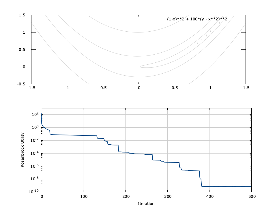
Figure [fig-optim-gradsearch]. gradsearch performance for 2-parameter Rosenbrock function \(f(x,y) = (1-x)^2 + 100(y-x^2)^2\) with a starting point of \((x_0,y_0)=(-0.1,1.4)\) . The minimum is located at \((1,1)\) .
[ref:fig-optim-gradsearch] depicts the performance of the gradient search for the Rosenbrock function, defined as\(f(x,y) = (1-x)^2 + 100(y-x^2)^2\) for input parameters \(x\) and \(y\) . The Rosenbrock function has a minimum at \((x,y)=(1,1)\) ; however the minimum lies in a deep valley which can be difficult to navigate. From the figure it is apparent that finding the valley is trivial, but convergence to the minimum is slow.