Equalization
API Keywords: equalization least mean squares LMS recursive least squares RLS eqlms eqrls
This section describes the equalizer module and the functionality of two digital linear adaptive equalizers implemented in liquid , LMS and RLS. Their interfaces are nearly identical; however their internal functionality is quite different. Specifically the LMS algorithm is less computationally complex but is slower to converge than the RLS algorithm.
System Description∞
Suppose a known transmitted symbol sequence\(\vec{d} = [ d(0), d(1), \ldots, d(N-1) ]\) which passes through an unknown channel filter \(\vec{h}_n\) of length\(q\) . The received symbol at time \(n\) is therefore
$$ y(n) = \sum\limits_{k=0}^{q-1}{h_n(k)d(n-k)} + \varphi(n) $$where \(\varphi(n)\) represents white Gauss noise. The adaptive linear equalizer attempts to use a finite impulse response (FIR) filter \(\vec{w}\) of length \(p\) to estimate the transmitted symbol, using only the received signal vector \(\vec{y}\) and the known data sequence \(\vec{d}\) , viz
$$ \hat{d}(n) = \vec{w}_n^T \vec{y}_n $$where \(\vec{y}_n = [ y(n), y(n-1),\ldots, y(n-p+1) ]^T\) . Several methods for estimating \(\vec{w}\) are known in the literature, and typically rely on iteratively adjusting \(\vec{w}\) with each input though a recursion algorithm. This section provides a very brief overview of two prevalent adaptation algorithms; for a more in-depth discussion the interested reader is referred to {cite:Proakis:2001,Haykin:2002}.
Least mean-squares equalizer (eqlms)∞
The least mean-squares (LMS) algorithm adapts the coefficients of the filter estimate using a steepest descent (gradient) of the instantaneous a priori error. The filter estimate at time \(n+1\) follows the following recursion
$$ \vec{w}_{n+1} = \vec{w}_{n} - \mu \vec{g}_n $$where \(\mu\) is the iterative step size, and\(\vec{g}_n\) the normalized gradient vector, estimated from the error signal and the coefficients vector at time \(n\) .
Recursive Least-squares Equalizer (eqrls)∞
The recursive least-squares (RLS) algorithm attempts to minimize the time-average weighted square error of the filter output, viz
$$ c(\vec{w}_n) = \sum\limits_{i=0}^{n}{ \lambda^{i-n} \left| d(i)-\hat{d}(i)\right|^2 } $$where the forgetting factor \(0\lt\lambda\leq 1\) which introduces exponential weighting into past data, appropriate for time-varying channels. The solution to minimizing the cost function \(c(\vec{w}_n)\) is achieved by setting its partial derivatives with respect to \(\vec{w}_n\) equal to zero. The solution at time \(n\) involves inverting the weighted cross correlation matrix for \(\vec{y}_n\) , a computationally complex task. This step can be circumvented through the use of a recursive algorithm which attempts to estimate the inverse using the a priori error from the output of the filter. The update equation is
$$ \vec{w}_{n+1} = \vec{w}_n + \Delta_{n} $$where the correction factor \(\Delta_{n}\) depends on \(\vec{y}_n\) and \(\vec{w}_n\) , and involves several \(p \times p\) matrix multiplications. The RLS algorithm provides a solution which converges much faster than the LMS algorithm, however with a significant increase in computational complexity and memory requirements.
Interface∞
The eqlms and eqrls have nearly identical interfaces so we will leave the discussion to the eqlms object here. Like most objects in liquid , eqlms follows the typical create() , execute() , destroy() life cycle. Training is accomplished either one sample at a time, or in a batch cycle. If trained one sample at a time, the symbols must be trained in the proper order, otherwise the algorithm won't converge. One can think of the equalizer object in liquid as simply a firfilt object (finite impulse response filter) which has the additional ability to modify its own internal coefficients based on some error criteria. Listed below is the full interface to the eqlms family of objects. While each method is listed for eqlms_cccf , the same functionality applies to eqlms_rrrf as well as the RLS equalizer objects ( eqrls_cccf and eqrls_rrrf ).
- eqlms_cccf_create(*h,n) creates and returns an equalizer object with \(n\) taps, initialized with the input array \(\vec{h}\) . If the array value is set to the NULL pointer then the internal coefficients are initialized to\(\{1,0,0,\ldots,0\}\) .
- eqlms_cccf_destroy(q) destroys the equalizer object, freeing all internally-allocated memory.
- eqlms_cccf_print(q) prints the internal state of the eqlms object.
- eqlms_cccf_set_bw(q,w) sets the bandwidth of the equalizer to \(w\) . For the LMS equalizer this is the learning parameter \(\mu\) which has a default value of 0.5. For the RLS equalizer the "bandwidth" is the forgetting factor\(\lambda\) which defaults to 0.99.
- eqlms_cccf_reset(q) clears the internal equalizer buffers and sets the internal coefficients to the default (those specified when create() was invoked).
- eqlms_cccf_push(q,x) pushes a sample \(x\) into the internal buffer of the equalizer object.
- eqlms_cccf_execute(q,*y) generates the output sample \(y\) by computing the vector dot product (see [ref:section-dotprod] ) between the internal filter coefficients and the internal buffer.
- eqlms_cccf_step(q,d,d_hat) performs a single iteration of equalization with an estimated output\(\hat{d}\) for an expected output \(d\) . The weights are updated internally defined by ([ref:eqn-equalization-lms_update] ) for the LMS equalizer and ([ref:eqn-equalization-rls_update] ) for the RLS equalizer.
- eqlms_cccf_get_weights(q,*w) returns the internal filter coefficients (weights) at the current state of the equalizer.
Here is a simple example:
#include <liquid/liquid.h>

int main() {
    // options
    unsigned int n=32;          // number of training symbols
    unsigned int p=10;          // equalizer order
    float mu=0.500f;            // LMS learning rate

    // allocate memory for arrays
    float complex x[n];         // received samples
    float complex d_hat[n];     // output symbols
    float complex d[n];         // traning symbols

    // ...initialize x, d_hat, d...

    // create LMS equalizer and set learning rate
    eqlms_cccf q = eqlms_cccf_create(NULL,p);
    eqlms_cccf_set_bw(q, mu);

    // iterate through equalizer learning
    unsigned int i;
    {
        // push input sample
        eqlms_cccf_push(q, x[i]);

         // compute output sample
        eqlms_cccf_execute(q, &d_hat[i]);

        // update internal weights
        eqlms_cccf_step(q, d[i], d_hat[i]);
    }

    // clean up allocated memory
    eqlms_cccf_destroy(q);
}
For more detailed examples, see examples/eqlms_cccf_example.c and examples/eqrls_cccf_example.c .
Blind Equalization∞
The equalizer interface above permits decision-directed equalization. This is a form of blind equalization where the data are not known, but the modulation scheme is. This type of equalization is useful for adapting to channel conditions, matched-filter ISI imperfections, and small timing offsets. Listed below is a basic program to equalize to a BPSK signal with unknown data.
#include <liquid/liquid.h>

int main() {
    // options
    unsigned int k=2;           // filter samples/symbol
    unsigned int m=3;           // filter semi-length (symbols)
    float beta=0.3f;            // filter excess bandwidth factor
    float mu=0.100f;            // LMS equalizer learning rate

    // allocate memory for arrays
    float complex * x;          // equalizer input sample buffer
    float complex * y;          // equalizer output sample buffer

    // ...initialize x, y...

    // create LMS equalizer (initialized on square-root Nyquist
    // filter prototype) and set learning rate
    eqlms_cccf q = eqlms_cccf_create_rnyquist(LIQUID_FIRFILT_RRC, k, m, beta, 0);
    eqlms_cccf_set_bw(q, mu);

    // iterate through equalizer learning
    unsigned int i;
    {
        // push input sample into equalizer and compute output
        eqlms_cccf_push(q, x[i]);
        eqlms_cccf_execute(q, &y[i]);

        // decimate output
        if ( (i%k) == 0 ) {
            // make decision and update internal weights
            float complex d_hat = crealf(y[i]) > 0.0f ? 1.0f : -1.0f;
            eqlms_cccf_step(q, d_hat, y[i]);
        }
    }

    // destroy equalizer object
    eqlms_cccf_destroy(q);
}
The equalizer filter is initialized with square-root raised-cosine coefficients (see [ref:section-filter-firdes-rnyquist] for details of square-root Nyquist filter designs). After computing each output symbol, the transmitted symbol is estimated and the equalizer adjusts its coefficients internally using the step() method. This can be easily combined with the linear modem object's modem_get_demodulator_sample() interface to return the estimated symbol after demodulation (see [ref:section-modem-digital] ).
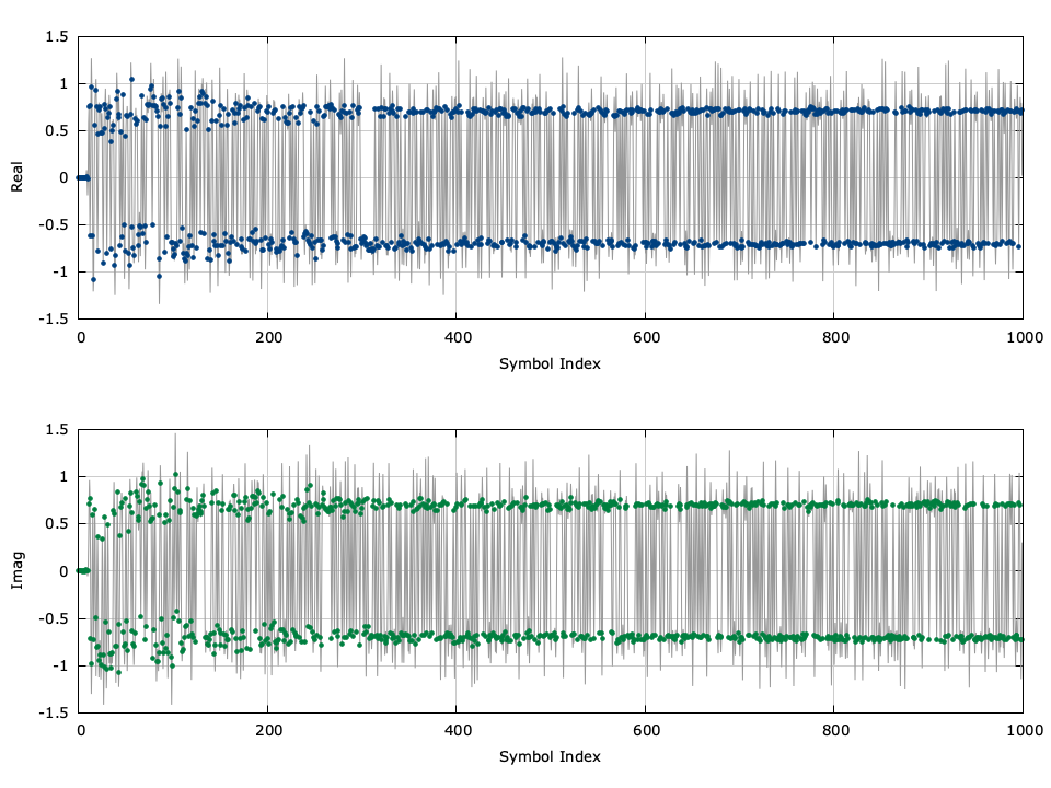
Figure [fig-equalization-eqlms-blind-time]. Equalizer output (time series)
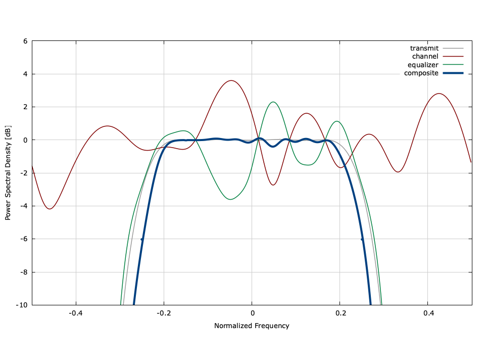
Figure [fig-equalization-eqlms-blind-freq]. Power Spectral Density
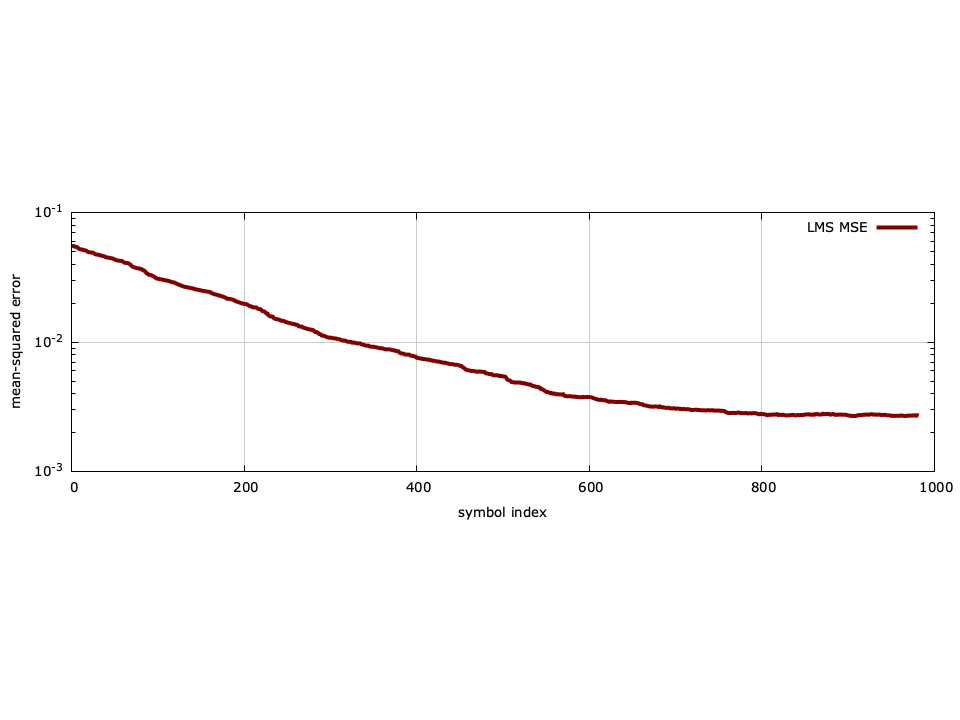
Figure [fig-equalization-eqlms-blind-mse]. Convergent mean-squared error
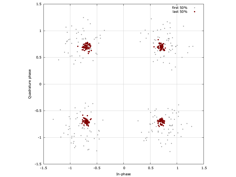
Figure [fig-equalization-eqlms-blind-const]. Constellation
Figure [fig-equalization-eqlms-blind]. Blind eqlms_cccf example, \(k=2\) samples/symbol