Writing a Phase-locked Loop in Straight C
By  on November 24, 2013
Keywords: phase-locked loop control PLL
Note: An updated (and simpler) version of this tutorial can be found here .
This tutorial explains how to write and simulate a phase-locked loop in the C programming language. You can download a tarball of this example which includes all the source code here: liquid_pll_example.tar.gz .
wget http://liquidsdr.org/blog/pll-howto/liquid_pll_example.tar.gz
tar -xvf liquid_pll_example.tar.gz
cd liquid_pll_example/
make
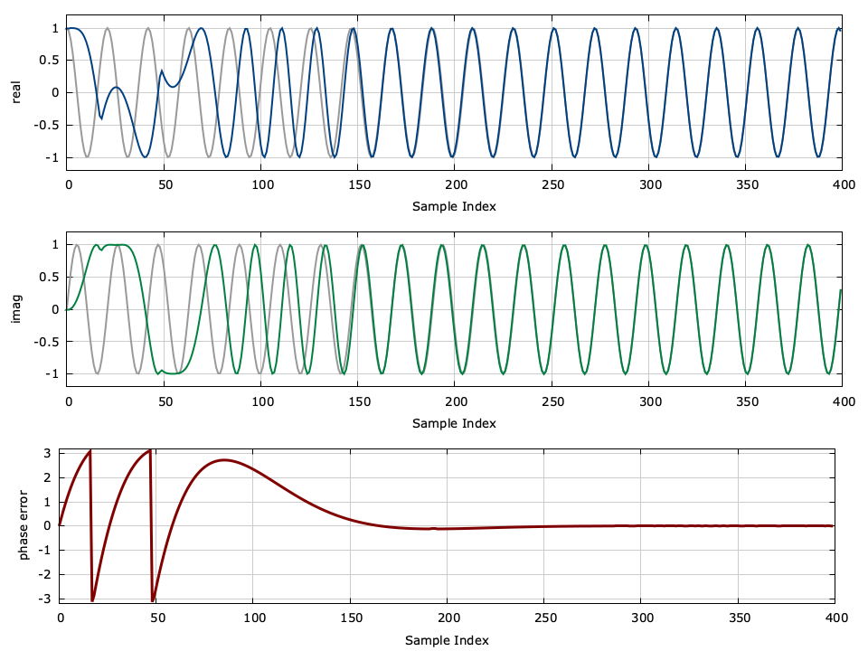
Figure [pll_example]. Phase-locked Loop Demonstration
Documentation for liquid-dsp already includes a basic tutorial for writing a phase-locked loop; however in that example the signal processing side of designing and implementing the filter has already been done for you. In this example, we will create a C implementation of a phase-locked loop without the dependencies on any external libraries, including liquid . I believe understanding the mechanics of something as fundamental as a phase-locked loop implemented using digital signal processing techniques in a low-level language is a great skill for any engineer to have.
Before You Begin...∞
For this example, you will need on your local machine:
- a text editor such as Vim
- a C compiler such as gcc
- a copy of Gnuplot or Octave for generating figures
- a terminal
The source code is provided up front in a single file with a full description of its operation. Once compiled, the program will run a simulation of the phase-locked loop, generating a data file which can be plotted using either Gnuplot or Octave . The problem statement and a brief theoretical description of phase-locked loops is given in the next section. A walk-through of the source code follows.
// https://liquidsdr.org/blog/pll-howto/ : simulate a phase-locked loop
#include <stdio.h>
#include <stdlib.h>
#include <complex.h>
#include <math.h>

int main() {
    // parameters
    float        phase_offset     = 0.00f;  // carrier phase offset
    float        frequency_offset = 0.30f;  // carrier frequency offset
    float        wn               = 0.01f;  // pll bandwidth
    float        zeta             = 0.707f; // pll damping factor
    float        K                = 1000;   // pll loop gain
    unsigned int n                = 400;    // number of samples

    // generate loop filter parameters (active PI design)
    float t1 = K/(wn*wn);   // tau_1
    float t2 = 2*zeta/wn;   // tau_2

    // feed-forward coefficients (numerator)
    float b0 = (4*K/t1)*(1.+t2/2.0f);
    float b1 = (8*K/t1);
    float b2 = (4*K/t1)*(1.-t2/2.0f);

    // feed-back coefficients (denominator)
    //    a0 =  1.0  is implied
    float a1 = -2.0f;
    float a2 =  1.0f;

    // print filter coefficients (as comments)
    printf("#  b = [b0:%12.8f, b1:%12.8f, b2:%12.8f]\n", b0, b1, b2);
    printf("#  a = [a0:%12.8f, a1:%12.8f, a2:%12.8f]\n", 1., a1, a2);

    // filter buffer
    float v0=0.0f, v1=0.0f, v2=0.0f;

    // initialize states
    float phi     = phase_offset;   // input signal's initial phase
    float phi_hat = 0.0f;           // PLL's initial phase

    // run basic simulation
    unsigned int i;
    float complex x, y;
    printf("# %6s %12s %12s %12s %12s %12s\n",
            "index", "real(x)", "imag(x)", "real(y)", "imag(y)", "error");
    for (i=0; i<n; i++) {
        // compute input sinusoid and update phase
        x = cosf(phi) + _Complex_I*sinf(phi);
        phi += frequency_offset;

        // compute PLL output from phase estimate
        y = cosf(phi_hat) + _Complex_I*sinf(phi_hat);

        // compute error estimate
        float delta_phi = cargf( x * conjf(y) );

        // print results to standard output
        printf("  %6u %12.8f %12.8f %12.8f %12.8f %12.8f\n",
            i, crealf(x), cimagf(x), crealf(y), cimagf(y), delta_phi);

        // push result through loop filter, updating phase estimate
        v2 = v1;  // shift center register to upper register
        v1 = v0;  // shift lower register to center register
        v0 = delta_phi - v1*a1 - v2*a2; // compute new lower register

        // compute new output
        phi_hat = v0*b0 + v1*b1 + v2*b2;
    }
    return 0;
}
Problem Statement∞
Wireless communications systems modulate the data signal with a high-frequency carrier before transmitting over the air. For many modulation schemes the receiver's oscillator needs to be locked in phase to that of the transmitter; however, in practice there is a small bit of residual carrier offset between the two. As its name implies, a phase-locked loop (PLL) is designed to lock the phase of an oscillator to the phase of a reference signal, providing a mechanism for synchronization on different platforms. In this example our input signal will be simply a complex sinusoid without noise or modulated information.
There are many types of phase-locked loops: digital (e.g. locking clocks together), analog (e.g. made with capacitors, transistors), etc. What we are designing here is really the digital equivalent of an analog PLL using digital signal processing rather than soldering together a circuit with discrete components. While the end result will be a discrete-time system, we will first design the PLL in the analog domain and then convert it to its digital counterpart.
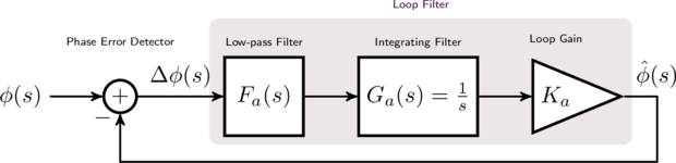
Figure [analog_pll_diagram]. scale:0.85 Continuous time analog phase-locked loop block diagram
[ref:analog_pll_diagram] depicts a simplified continuous-time analog PLL. We can think of the input to the system as being an unknown phase \(\phi\) , possibly corrupted by noise, while the output of is an estimate of this phase, \(\hat{\phi}\) . As you can see from [ref:analog_pll_diagram] , there are just two main components to the phase-locked loop: the phase error detector and the loop filter. In general the phase error detector simply computes the difference between the input and estimated phases while the loop filter removes much of the noise and tracks to the time-varying input phase. Much of the analysis in this tutorial will focus on designing the loop filter in [ref:analog_pll_diagram] .
Designing the Loop Filter (Analog Domain)∞
The loop filter consists of three components: a first-order low-pass filter \(F_a(s)\) , a first-order integrator \(G_a(s)\) , and a constant loop gain \(K_a\) (the subscript \(a\) denotes "analog"). We can derive the analog transfer function \(H_a(s)=\hat{\phi}(s) / \phi(s)\) considering that \(\phi(s)\) is the input and \(\hat{\phi}(s)\) is the output:
$$ \begin{array}{lll} \hat{\phi}(s) & = & \Delta\phi(s) F_a(s) G_a(s) K_a \\ & = & \Bigl[ \phi(s) - \hat{\phi}(s) \Bigr] F_a(s) G_a(s) K_a \\ \hat{\phi}(s)\Bigl[ 1 + F_a(s) G_a(s) K_a \Bigr] & = & \phi(s) F_a(s) G_a(s) K_a \\ H_a(s) & \triangleq & \frac{\hat{\phi}(s)}{\phi(s)} \\ & = & \frac{F_a(s) G_a(s) K_a}{1 + F_a(s) G_a(s) K_a} \end{array} $$There are several well-known options for designing the first-order low-pass filter \(F_a(s)\) . In particular we are interested in getting the denominator of \(H_a(s)\) to the standard form
$$ s^2 + 2\zeta\omega_n s + \omega_n^2 $$where \(\omega_n\) is the natural frequency of the filter and \(\zeta\) is the damping factor. This simplifies analysis of the overall transfer function and allows the parameters of \(F_a(s)\) to ensure stability. We are now free to choose the low pass filter \(F_a(s)\) . There are several possibilities, but for this example we will use the active "proportional plus integration" (PI) which has a loop filter
$$ F_a(s) = \frac{1 + \tau_2 s}{\tau_1 s} $$where \(\tau_1\) and \(\tau_2\) are also parameters relating to the damping factor and natural frequency. This yields a closed-loop phase-locked loop transfer function:
$$ H_a(s) = \frac{ \frac{K_a}{\tau_1} (1 + s\tau_2) } { s^2 + s\frac{K_a\tau_2}{\tau_1} + \frac{K_a}{\tau_1} } $$Converting the denominator of [ref:eqn:loop_filter_Ha] into standard form in [ref:eqn:pll_denominator_standard_form] yields the following equations for \(\tau_1\) and \(\tau_2\) :
$$ \omega_n = \sqrt{\frac{K_a}{\tau_1}} \,\,\,\,\,\, \zeta = \frac{\omega_n \tau_2}{2} \rightarrow \tau_1 = \frac{K_a}{\omega_n^2} \,\,\,\,\,\, \tau_2 = \frac{2\zeta}{\omega_n} $$We are left with a loop filter that simply has three parameters:
- \(\omega_n\) : the bandwidth of the loop filter
- \(\zeta\) : the loop filter's damping factor (typically \(\zeta=1/\sqrt{2} \approx 0.707\) )
- \(K_a\) : the loop filter's gain (typically \(K_a\) is very large, on the order of 1,000)
The values \(\tau_1\) and \(\tau_2\) are derived from \(\omega_n\) , \(\zeta\) , and\(K_a\) .
Loop Filter: Converting to Digital∞
Now that we have a design for the analog filter \(H_a(s)\) in[ref:eqn:loop_filter_Ha] , we need to convert it to a digital equivalent\(H_d(z)\) so that we may simulate the PLL using discrete signal processing. To accomplish this we will use the bilinear \(z\) -transform which replaces \(s\) with \(\frac{1}{2}\frac{1-z^{-1}}{1+z^{-1}}\) (follow this link for a detailed description). Consequently, because \(H_a(s)\) is a second-order analog filter,\(H_d(z)\) will be a second-order digital filter of the form
$$ H_d(z) = \frac{\hat{\phi}(z)}{\phi(z)} = \frac{ b_0 + b_1 z^{-1} + b_2 z^{-2}} { 1 + a_1 z^{-1} + a_2 z^{-2}} $$where \(b_0\) , \(b_1\) , and \(b_2\) are known as the feed-forward coefficients and\(a_1\) and \(a_2\) are known as the feedback coefficients (note that typically the coefficients in \(H_d(z)\) are normalized such that \(a_0=1\) ). Figure [ref:iirfilt_sos_diagram] below provides a general block diagram for a basic \(2^{nd}\) -order filter.

Figure [iirfilt_sos_diagram]. scale:0.7 Direct form II realization for a \(2^{nd}\) order recursive (infinite impulse response) filter
where the \(z^{-1}\) blocks represent a single sample delay and the\(v_0\) , \(v_1\) , and \(v_2\) nodes represent memory registers.
Taking the bilinear \(z\) -transform of \(H_a(s)\) in[ref:eqn:loop_filter_Ha] gives the digital filter
$$ H_d(z) = H_a(s)\Bigl.\Bigr|_{s = \frac{1}{2}\frac{1-z^{-1}}{1+z^{-1}}} = 2 K_a \frac{ (1+\tau_2/2) + 2 z^{-1} + ( 1 - \tau_2/2)z^{-2} } { \tau_1/2 -\tau_1 z^{-1} + (\tau_1/2)z^{-2} } $$Putting \(H_d(z)\) in systematic form (scaling both the numerator an denominator by \(\tau_1/2\) ) gives:
$$ H_d(z) = \frac{4 K_a}{\tau_1} \left[ \frac{ (1+\tau_2/2) + 2 z^{-1} + ( 1 - \tau_2/2)z^{-2} } { 1 - 2 z^{-1} + z^{-2} } \right] $$This provides the set of digital filter coefficients:
$$ \begin{array}{llllll} b_0 & = & \frac{4 K_a}{\tau_1} (1+\tau_2/2), & a_0 & \triangleq & 1 \\ b_1 & = & \frac{8 K_a}{\tau_1}, & a_1 & = & -2 \\ b_2 & = & \frac{4 K_a}{\tau_1} ( 1 - \tau_2/2), & a_2 & = & 1 \end{array} $$We can verify the stability of the filter by ensuring that the filter poles (the complex roots of the polynomial in the denominator with respect to\(z^{-1}\) ) are within the unit circle. A careful inspection of the polynomial in the denominator of[ref:eqn:loop_filter_Hd] reveals that the two conjugate roots\(p_d\) and \(p_d^*\) are not only on the unit circle, but they are also both real-valued:
$$ \begin{array}{lll} 1 - 2 z^{-1} + z^{-2} & = & (1 - p_d z^{-1}) (1 - p_d^* z^{-1}) \\ p_d & = & 1 \\ p_d^* & = & 1 \end{array} $$The full digital phase-locked loop can be found in [ref:digital_pll_diagram] , below.
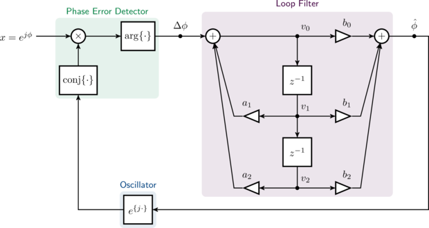
Figure [digital_pll_diagram]. Full digital phase-locked loop
Getting the Source Code∞
While I have provided a copy of the source code at the top of this document, you may simply download a tarball that includes the following files:
- pll_example.c : the source code for the simulation
- pll_example.gnuplot : a Gnuplot script to convert the results of the simulation into [ref:pll_example]
- pll_example.m : an Octave/MATLAB script as an alternative to Gnuplot for generating a figure
- index.pdf : a .pdf version of this document
- makefile : a make script to automatically build and run the simulation, and generate a plot of the results
You can download the tarball by either clicking on this link: liquid_pll_example.tar.gz . or using wget :
wget http://liquidsdr.org/blog/pll-howto/liquid_pll_example.tar.gz
or using curl :
curl -O http://liquidsdr.org/blog/pll-howto/liquid_pll_example.tar.gz
Unzip the tarball, move into the directory, and then build the example
tar -xvf liquid_pll_example.tar.gz
cd liquid_pll_example/
make
If successful, the make command will compile the program, execute it while piping the results to pll_example.dat , and then run gnuplot to create an image file pll_example.png to display the results.
Source Code Breakdown∞
The program initially sets the parameters for the simulation, including the carrier phase and frequency offsets, the phase-locked loop filter specifications, and the number of samples to run. Note that the frequency is relative to an unspecified sample rate, so the maximum is \(\pi\) and the minimum is \(-\pi\) . Typically the frequency offset is relatively small, usually less than\(\pm 0.5\) .
Initializing the variables to describe the loop filter can be a bit tricky. We need to allocate three sets of variables for the filter: the feed-forward coefficients ( b0 , b1 , and b2 ) the feedback coefficients ( a1 and a2 ) and the filter's internal memory state ( v0 , v1 , and v2 ) The values for the coefficients were computed in[ref:eqn:loop_filter_coefficients] and can be specified directly. The filter's memory state variables should be initialized each to zero.
The program loop steps through the operation as given in[ref:digital_pll_diagram] :
- Compute the input sinusoid \(x\) and update the input phase \(\phi\)
- Compute PLL output signal \(y\) from output phase \(\hat{\phi}\)
- Compute phase error approximation \(\Delta\phi\)
- Push the phase error through loop filter and update PLL output phase
Inside the loop the program computes the input signal x as \(x=e^{j\hat{\phi}}\) and updates its phase. PLL output y is derived from its phase estimate as \(y=e^{j\hat{\phi}}\) . The best estimate for phase error is the angle difference between \(x\) and \(y\) , or simply \(\Delta\phi = \arg\{x y^*\}\) ; however you could alternatively use the imaginary component of \(xy^*\) at a slight performance cost. The next step is to update the loop filter from this phase error. This can be a bit tricky. In the direct form II of the recursive filter (see [ref:iirfilt_sos_diagram] ), we first need to advance the register state by dropping the oldest sample, v0 , and shifting the newer two samples ( v1 and v2 ) down. The new lower register value v0 is computed simply as\(v_0=\Delta\phi - v_1 a_1 - v_2 a_2\) . Finally the loop filter output \(\hat{\phi}\) can be computed as\(\hat{\phi} = v_0 b_0 + v_1 b_1 + v_2 b+2\) . For each step of the loop the program saves the result to a file that can later be plotted with Gnuplot .
You can compile the binary by running gcc from the command line:
gcc -o pll_example pll_example.c -Wall -O2 -lc -lm
Run the resulting pll_example program and pipe the output to pll_example.dat :
./pll_example > pll_example.dat
The output file should contain data that looks something like this:
#  b = [b0:  0.02868000, b1:  0.00080000, b2: -0.02788000]
#  a = [a0:  1.00000000, a1: -2.00000000, a2:  1.00000000]
#  index      real(x)      imag(x)      real(y)      imag(y)        error
       0   1.00000000   0.00000000   1.00000000   0.00000000   0.00000000
       1   0.95533651   0.29552022   1.00000000   0.00000000   0.29999998
       2   0.82533562   0.56464249   0.99996299   0.00860389   0.59139597
       3   0.62160993   0.78332692   0.99940807   0.03440245   0.86559081
       4   0.36235771   0.93203908   0.99702549   0.07707223   1.12285137
     ...
     394   0.38084957  -0.92463702   0.37742791  -0.92603898   0.00369773
     395   0.63709074  -0.77078879   0.63436598  -0.77303284   0.00352991
     396   0.83642137  -0.54808688   0.83443946  -0.55109966   0.00360624
     397   0.96103549  -0.27642506   0.96004522  -0.27984500   0.00356043
     398   0.99980140   0.01992950   0.99986923   0.01617134   0.00375878
     399   0.94925624   0.31450379   0.95041740   0.31097704   0.00371299
The included Gnuplot script (listed below) will generate an output image pll_example.png :
# pll_example.gnuplot : configuration for output plot

reset                                   # reset
set size ratio 0.2                      # set relative size of plots
set xlabel 'Sample Index'               # set x-axis label for all plots
set grid xtics ytics                    # grid: enable both x and y lines
set grid lt 1 lc rgb '#cccccc' lw 1     # grid: thin gray lines
set multiplot layout 3,1 scale 1.0,1.0  # set three plots for this figure

# real
set ylabel 'real'                       # set y-axis label
set yrange [-1.2:1.2]                   # set plot range
plot 'pll_example.dat' using 1:2 with lines lt 1 lw 2 lc rgb '#999999' notitle ,\
     'pll_example.dat' using 1:4 with lines lt 1 lw 2 lc rgb '#004080' notitle

# imag
set ylabel 'imag'                       # set y-axis label
set yrange [-1.2:1.2]                   # set plot range
plot 'pll_example.dat' using 1:3 with lines lt 1 lw 2 lc rgb '#999999' notitle ,\
     'pll_example.dat' using 1:5 with lines lt 1 lw 2 lc rgb '#008040' notitle

# phase error
set ylabel 'phase error'                # set y-axis label
set yrange [-3.2:3.2]                   # set plot range
plot 'pll_example.dat' using 1:6 with lines lt 1 lw 3 lc rgb '#800000' notitle

unset multiplot
Generate the figure by invoking gnuplot from the command-line terminal:
gnuplot -e 'set terminal png' pll_example.gnuplot > pll_example.png
If you prefer, you could also load the data and plot it using Octave or MATLAB with the suppled pll_example.m script:
% pll_example.m : simple Octave script to plot the results of pll_example.c

clear all;
close all;

% load data into single vector
v = load('pll_example.dat');
index = v(:,1);             % index
x     = v(:,2) + 1i*v(:,3); % input sinusoid
y     = v(:,4) + 1i*v(:,5); % output sinusoid
dphi  = v(:,6);             % phase error

figure;

% plot real components
subplot(3,1,1),
  plot(index, real(x), real(y));
  xlabel('Sample Index');
  ylabel('real');
  grid on;

% plot imaginary components
subplot(3,1,2),
  plot(index, imag(x), imag(y));
  xlabel('Sample Index');
  ylabel('imag');
  grid on;

% plot phase error
subplot(3,1,3),
  plot(index, dphi);
  xlabel('Sample Index');
  ylabel('phase error');
  grid on;
The included makefile simplifies the compilation process by only running necessary operations.
# makefile : simple makefile for building and running a phase-locked loop

# default target
all : pll_example.png

# main program target
pll_example : pll_example.c
	gcc -o $@ $< -Wall -O2 -lc -lm

# output data file
pll_example.dat : pll_example
	./pll_example > pll_example.dat

# output figure (.png)
pll_example.png : pll_example.gnuplot pll_example.dat
	gnuplot -e 'set terminal png size 800,700' $< > $@

# remove generated files
clean :
	rm -f pll_example
	rm -f pll_example.dat
	rm -f pll_example.png
That is, you can simply generate the output pll_example.png figure simply by executing
make
Play around with changing the simulation parameters and see how the PLL's response changes. With the default settings it takes about 175 samples before the PLL locks on to the input phase of the signal; how long does it take if you increase the loop filter bandwidth \(\omega_n\) to 0.02f ?
Revisions∞
- 27 Dec 2017 : Fixing typo in denominator in [ref:eqn:loop_filter_Ha] ; thanks to E. Ponce for pointing this out