Least Mean-Squares Equalizer
By  on December 29, 2018
Keywords: least mean squares LMS equalizer equalization adaptive filter
This tutorial provides an overview of a very simple fininite impulse response least mean-squares equalizer simulation. This is part of my "DSP in 50 lines of C" series.
// liquidsdr.org/blog/lms-equalizer/
#include <stdlib.h>
#include <stdio.h>
#include <math.h>
#include <complex.h>

int main() {
    unsigned int M           = 1 << 3;  // phase-shift keying mod. order
    unsigned int num_symbols = 1200;    // number of symbols to simulate
    unsigned int w_len       = 13;      // equalizer length
    float        mu          = 0.05f;   // equalizer learning rate
    float        alpha       = 0.60f;   // channel filter bandwidth

    // create and initialize arrays
    unsigned int  n, i, buf_index=0;
    float complex w[w_len];             // equalizer coefficients
    float complex b[w_len];             // equalizer buffer
    for (i=0; i<w_len; i++) w[i] = (i == w_len/2) ? 1.0f : 0.0f;
    for (i=0; i<w_len; i++) b[i] = 0.0f;

    float complex x_prime = 0;
    for (n=0; n<num_symbols; n++) {
        // 1. generate random transmitted phase-shift keying symbol
        float complex x = cexpf(_Complex_I*2*M_PI*(float)(rand() % M)/M);

        // 2. compute received signal and store in buffer
        float complex y = sqrt(1-alpha)*x + alpha*x_prime;
        x_prime = y;
        b[buf_index] = y;
        buf_index = (buf_index+1) % w_len;

        // 3. compute equalizer output
        float complex r = 0;
        for (i=0; i<w_len; i++)
            r += b[(buf_index+i)%w_len] * conjf(w[i]);

        // 4. compute 'expected' signal (blind), skip first w_len symbols
        float complex e = n < w_len ? 0.0f : r - r/cabsf(r);

        // 5. adjust equalization weights
        for (i=0; i<w_len; i++)
            w[i] = w[i] - mu*conjf(e)*b[(buf_index+i)%w_len];

        // print resulting symbols to screen
        printf("%8.3f %8.3f",   crealf(y), cimagf(y)); // received
        printf("%8.3f %8.3f\n", crealf(r), cimagf(r)); // equalized
    }
    return 0;
}
Overview∞
Wide-band single-carrier systems commonly suffer from distortion across the modulated band, often caused by imperfect transmit or receive filters in hardware or multi-path channel effects. This manifests as inter-symbol interference in the received constellation causing an increase in errors if left uncorrected. Equalization attempts to remove these effects by dynamically adjusting the coefficients of a filter to minimize some cost function, often the mean-squared error. With a good equalizer the linear effects of the channel can be virtually removed. Non-linear effects such as noise, interference, and clipping can be mitigated if the equalizer is designed properly, but only up to a limit.
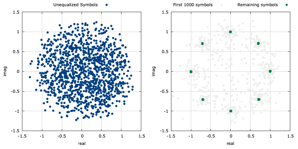
Figure [equalizer]. The results of this simulation with the symbols before (left) and after (right) equalization.
For the sake of simplicity, we will operate at complex baseband, sampled at one sample per symbol. In practice operating at a higher sample rate is preferred because the equalizer can prevent aliasing before down-sampling, further reducing distortion. The figure above demonstrates the input and output symbols simulated in the above source code.
Description of Operation∞
Suppose a transmitted symbol sequence\(\vec{x} = [ x(1), x(2), \ldots, x(N) ]\) passes through an unknown and time-varying channel. The receiver observes a sequence of symbols\(\vec{y} = [ y(1), y(2), \ldots, y(N) ]\) which are correlated due to the channel filter and noisy due to an additive random process. The adaptive linear equalizer attempts to use a finite impulse response (FIR) filter \(\vec{w}\) of length \(p\) to estimate the transmitted symbols using only the received signal vector \(\vec{y}\) and partial knowledge of the known data sequence \(\vec{x}\) . Several methods for estimating the weights in \(\vec{w}\) are known in the literature, and typically rely on iteratively adjusting \(\vec{w}\) with each input though a recursion algorithm. The method is described in the documentation on equalizers in liquid for both the least mean-squared (LMS) and recursive least-squared (RLS) algorithms. Due it its simplicity and relatively low complexity, this post will focus on the LMS equalizer.
The least mean-squares (LMS) algorithm adapts the coefficients of the filter estimate using a steepest descent (gradient) of the instantaneous a priori error. The filter estimate at time \(n+1\) follows the following recursion
$$ \vec{w}_{n+1} = \vec{w}_{n} - \mu \vec{\nabla}_n $$where \(\mu\) is the iterative step size, and\(\vec{\nabla}_n\) the normalized gradient vector, estimated from the error signal and the coefficients vector at time \(n\) .
Often in practice the receiver has no knowledge of the transmitted sequence\(\vec{x}\) and so an estimate must be made for the gradient vector at each time step. Furthermore, the receiver might have no knowledge of even the transmitter's modulation scheme and so the receiver must make an estimate completely in the blind. In this situation a relatively good error value is just the deviation from the equalizer output from its nearest point on the unit circle:
$$ e(n) \triangleq r(n) - \frac{r(n)}{|r(n)|} $$where \(r(n)=[y(n-p+1),\ldots,y(n)]\cdot\vec{w}^H\) is the output of the equalizer at time \(n\) . This is effectively saying that the equalizer should have produced a symbol that has the same phase as \(r(n)\) but lies on the unit circle. From this, a reasonable estimate of the error gradient is simply the last \(p\) received symbols scaled by the conjugate of this complex error signal
$$ \vec{\nabla}_n \approx e^*(n) [y(n-p+1),\ldots,y(n)]^T $$Coding it up∞
The source code above is organized as usual with simulation options at the top, followed by value initialization and the main loop. Within the loop there are five steps for simulating the equalizer:
- The time index is set to \(n\) and the transmitter generates a random\(M\) -ary phase-shift keying symbol \(x(n) = \exp\{j2\pi k/M\}\) for \(k \in \{0,1,\ldots,M-1\}\)
- The received symbol \(y(n)\) is computed from the channel filter (in this case a single-pole recursive filter for simplicity) and the receiver stores it at the end of its buffer,\(\vec{b}_n = [ y(n-p+1), \ldots, y(n) ]^T\)
- The receiver uses its current set of weights \(\vec{w}_n\) to compute the output of the equalizer \(r(n) = \vec{b}_n^T \vec{w}_n\)
- A blind estimate of the error signal is computed by finding the vector between the equalizer output and the closest corresponding value on the unit circle, \(e(n) = r(n) - r(n)/|r(n)|\)
- The equalizer weights are adjusted according to the estimated error signal from the equalizer otuput and the last \(p\) received symbols, viz\(\vec{w}_{n+1} = \vec{w}_n - \mu e^*(n) \vec{b}_n\)
Compile equalizer.c above and run the program with:
gcc -Wall -O2 -lm -lc -o equalizer.c -o equalizer
./equalizer
...which should produce the following output.
   0.447   -0.447   0.000    0.000
   0.716    0.179   0.000    0.000
   0.877    0.555   0.000    0.000
   0.526    0.965   0.000    0.000
   0.316    1.212   0.000    0.000
   0.822    0.727   0.000    0.000
   1.126    0.436   0.447   -0.447
   0.675   -0.371   0.716    0.179
     ...
   0.627   -0.245   0.005   -1.001
  -0.257   -0.147   0.710   -0.700
   0.293   -0.535   0.703    0.707
   0.623   -0.768   0.006   -0.994
   0.374   -1.093   0.700    0.709
   0.672   -1.103  -0.700   -0.709
The first two columns are the real and imaginary components of the input symbols, respectively. The third and fourth columns are the real/imag of the output. Plotting these symbols gives the figure near the top of this post.
Considerations∞
This is a blind estimation method. What happens when the modulation scheme isn't phase-shift keying, but quadrature amplitude modulation ? As it turns out, this blind estimator works quite well for most digital modulation types provided that the underlying data are sufficiently random. Of course the performance is not as good as a decision-directed method (where knowledge of the underlying modulation scheme is known), or when a known transmitted sequence is used. Furthermore, the blind estimation method used here cannot compensate for unknown phase offsets.