Random Number Generators

The random module in liquid includes a comprehensive set of random number generators useful for simulation of wireless communications channels, particularly for generating noise as well as fading channels. This includes the uniform, normal, circular (complex) Gaussian, Rice-\(K\) , and Weibull distributions.

Uniform∞

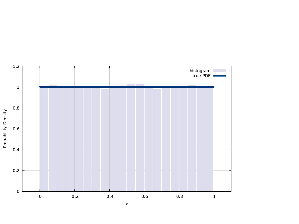
The uniform random variable generator in liquid simply generates a number evenly distributed in \([0,1)\) . Internally liquid uses the standard rand() method for generating random integers and then divides by RAND_MAX , the maximum number that can be generated. The probability density function is defined as

$$ f_X(x) = \begin{cases} 1 & \text{if $0 \leq x \lt 1$} \\ 0 & \text{else}. \end{cases} $$

The uniform random number generator is the basis for generating most other distributions in liquid .

Uniform random number generator interface:
float randf();
float randf_pdf(float _x);
float randf_cdf(float _x);

Normal (Gaussian)∞

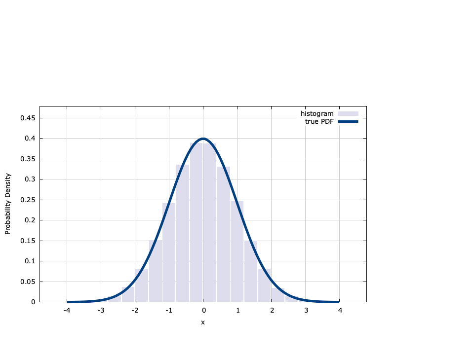
The normal (or Gauss) distribution has a probability density function defined as

$$ f_X(x;\sigma,\eta) = \frac{1}{\sigma \sqrt{2 \pi}} e^{-\left(x-\eta\right)^2/{2\sigma^2}} $$

liquid generates normal random variables using the Box-Muller method. If \(U_1\) and \(U_2\) are uniform random variables with a distribution defined by [ref:eqn-random-uniform-pdf] , then\(X_1 = \sqrt{-2\ln(U_1)} \sin\left(2 \pi U_2\right)\) and\(X_2 = \sqrt{-2\ln(U_1)} \cos\left(2 \pi U_2\right)\) are independent normal random variables with a mean of zero and a unity standard deviation (\(X_1, X_2 \sim N(0,1)\) ).

Normal (Gauss) random number generator interface:
float randnf();
float randnf_pdf(float _x,
                 float _eta,
                 float _sigma);
float randnf_cdf(float _x,
                 float _eta,
                 float _sigma);

Exponential∞

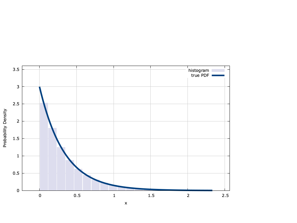
The exponential distribution has a probability density function defined as

$$ f_X(x;\lambda) = \lambda e^{-\lambda x} $$

liquid generates exponential random variables by inverting the cumulative distribution function, viz

$$ F_X(x;\lambda) = 1 - e^{-\lambda x} $$

Specifically if \(U\) is uniform random variable with a distribution defined by [ref:eqn-random-uniform-pdf] then\(X = -\ln U / \lambda\) has an exponential distribution defined by[ref:eqn-random-exponential-cdf] .

Exponential random number generator interface:

float randexpf(float _lambda);
float randexpf_pdf(float _x, float _lambda);
float randexpf_cdf(float _x, float _lambda);

Weibull∞

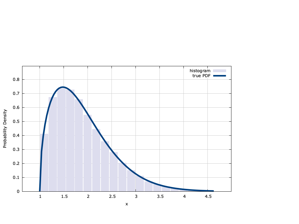
The Weibull distribution has a probability density function defined by

$$ f_X(x;\alpha,\beta,\gamma) = \begin{cases} \frac{\alpha}{\beta} \left( \frac{x-\gamma}{\beta} \right)^{\alpha-1} \exp\Bigl\{ -\left( \frac{x-\gamma}{\beta} \right)^\alpha \Bigr\} & \text{$x \ge \gamma$} \\ 0 & \text{else}. \end{cases} $$

where\(\alpha\) is the shape parameter,\(\beta\) is the scale parameter, and\(\gamma\) is the threshold parameter. liquid generates Weibull random variables by inverting the cumulative distribution function, viz

$$ F_X(x;\alpha,\beta,\gamma) = \begin{cases} 1 - \exp\left\{ -\left(\frac{x-\gamma}{\beta}\right)^\alpha \right\} & x \ge \gamma \\ 0 & \text{else}. \end{cases} $$

Specifically if \(U\) is uniform random variable with a distribution defined by [ref:eqn-random-uniform-pdf] then\(X = \gamma + \beta\left[ \ln\left(1 - U\right) \right]^{1/\alpha}\) has a Weibull distribution defined by [ref:eqn-random-weibull-cdf] .

Weibull random number generator interface:

float randweibf(float _alpha,
                float _beta,
                float _gamma);
float randweibf_pdf(float _x,
                    float _alpha,
                    float _beta,
                    float _gamma);
float randweibf_cdf(float _x,
                    float _alpha,
                    float _beta,
                    float _gamma);

Gamma∞

The gamma distribution has a probability density function defined by

$$ f_X(x;\alpha,\beta) = \begin{cases} \frac{ x^{\alpha-1} }{ \Gamma(\alpha) \beta^\alpha } e^{-x / \beta} & x \ge 0 \\ 0 & \text{else}. \end{cases} $$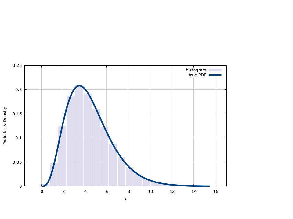

Gamma random number generator interface:

float randgammaf(float _alpha,
                 float _beta);
float randgammaf_pdf(float _x,
                     float _alpha,
                     float _beta);
float randgammaf_cdf(float _x,
                     float _alpha,
                     float _beta);

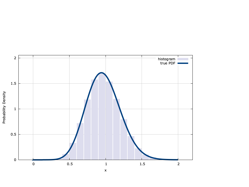
Nakagami-m∞

The Nakagami-\(m\) distribution is a versatile stochastic model for modeling radio links {cite:Braun:1991} and has often been regarded as the best distribution to model land mobile propagation due to its ability to describe fading situations worse than Rayleigh, including one-sided Gaussian {cite:Simon:1998}. Empirical evidence regarding the efficacy the Nakagami-\(m\) distribution has on fading profiles been presented in {cite:Turin:1980, Suzuki:1977}. Thus statistical inference of the Nakagami-\(m\) fading parameters are of interest in the design of adaptive radios such as optimized transmit diversity modes {cite:Cavers:1999, Ko:2003} and adaptive modulation schemes {cite:Catreux:2002}. The Nakagami-\(m\) probability density function is given by {cite:Papoulis:2002}

$$ f_X(x;m,\Omega) = \begin{cases} \frac{2}{\Gamma(m)} \left( \frac{m}{\Omega} \right)^m x^{2m-1} e^{ -(m/\Omega)x^2} & x \ge 0 \\ 0 & \text{else}. \end{cases} $$

where\(m \ge 1/2\) is the shape parameter and\(\Omega \gt 0\) is the spread parameter. Nakagami-\(m\) random numbers are generated from the gamma distribution. Specifically if \(R\) follows a gamma distribution defined by[ref:eqn-random-gamma-pdf] with parameters \(\alpha\) and \(\beta\) , then \(X=\sqrt{R}\) has a Nakagami-\(m\) distribution with\(m=\alpha\) and \(\Omega=\beta/\alpha\) .

Nakagami random number generator interface:

float randnakmf(float _m,
                float _omega);
float randnakmf_pdf(float _x,
                    float _m,
                    float _omega);
float randnakmf_cdf(float _x,
                    float _m,
                    float _omega);

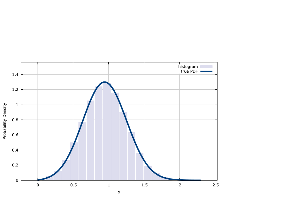
Rice-K∞

The Rice-\(K\) multi-path channel models a fading envelope by assuming a line of sight (LoS) component to the multi-path elements summed at the receiver. The complex path gain at a particular frequency consists of a fixed (LoS) and fluctuating (diffuse) components. When assuming a narrowband complex Gaussian stochastic process, the time-varying envelope will exhibit a Rice distribution where the \(K\) factor is the power ratio of the LoS and diffuse components (often referred to in dB) and thus is commonly used to describe fading environments. The Rice-\(K\) distribution has a probability density function defined as

$$ f_R(r;K,\Omega) = \frac{2(K+1)r}{\Omega} \exp\left\{-K-\frac{(K+1)r^2}{\Omega}\right\} I_0\left( 2r\sqrt{\frac{K(K+1)}{\Omega}} \right) $$

where \(\Omega=E\left\{R^2\right\}\) is the average signal power and \(K\) is the fading factor (shape parameter). liquid generates Rice-\(K\) random variables using two independent normal random variables. Specifically if\(X_0 \sim N(0,\sigma)\) and\(X_1 \sim N(s,\sigma)\) then\(R = \sqrt{X_0^2 + X_1^2}\) has follows a Rice-\(K\) distribution defined by[ref:eqn-random-ricek-pdf] where\(s = \sqrt{\frac{\Omega K}{K+1}}\) and\(\sigma = \sqrt{\frac{\Omega}{2(K+1)}}\) .

Rice-\(K\) random number generator interface:

float randricekf(float _m,
                 float _omega);
float randricekf_pdf(float _x,
                     float _K,
                     float _omega);
float randricekf_cdf(float _x,
                     float _K,
                     float _omega);

Data scrambler∞

Physical layer synchronization of received waveforms relies on independent and identically distributed underlying data symbols. If the message sequence, however, is too repetitive (such as ' 00000.... ' or ' 11001100.... ') and the modulation scheme is BPSK, the synchronizer probably won't be able to recover the symbol timing because adjacent symbols are too similar. This is a result of spectral correlation introduced which can prevent physical layer synchronization techniques from tracking or even acquisition. Having said that, certain patterns are beneficial to synchronization and actually help the receiver track to the incoming signal, however these are usually only introduced as a preamble to a frame or packet where the receiver knows what to expect. It is therefore imperative to increase the short-term entropy of the underlying data to prevent the receiver from losing its lock on the signal. The data scrambler routine attempts to "whiten" the data sequence with a bit mask in order to achieve maximum entropy.

interface∞

The data scrambler has two methods, described here:

• scramble_data() takes an input sequence of data and scrambles the bits by applying a periodic mask. The first argument is a pointer to the input data array; the second argument is its length (number of bytes).
• unscramble_data() takes an input sequence of data and unscrambles the bits by applying the reverse mask applied by scramble_data() . Just like scramble_data() , the first argument is a pointer to the input data array; the second argument is its length (number of bytes).

See examples/scramble_example.c for a full example of the interface.

Here is a basic example of data scrambling in liquid:

#include <liquid/liquid.h>
#include <string.h>

int main() {
    // number of data bytes
    unsigned int  msg_len = 1234;

    // message array
    unsigned char message[msg_len];

    // ... initialize message ...

    // scramble input
    scramble_data(message, msg_len);

    // unscramble result
    unscramble_data(message, msg_len);

    return 0;
}