Numerically-Controlled Oscillator (nco)
API Keywords: numerically controlled oscillator NCO voltage controlled oscillator VCO nco_crcf nco_rrrf
The nco object implements an oscillator with two options for internal phase precision: LIQUID_NCO and LIQUID_VCO . The LIQUID_NCO implements a numerically-controlled oscillator that uses a look-up table to generate a complex sinusoid while the LIQUID_VCO implements a "voltage-controlled" oscillator that uses the sinf and cosf standard math functions to generate a complex sinusoid.
Description of operation∞
The nco object maintains its phase and frequency states internally. Various computations--such as mixing--use the phase state for generating complex sinusoids. The phase \(\theta\) of the nco object is updated using the nco_crcf_step() method which increments \(\theta\) by \(\Delta\theta\) , the frequency. Both the phase and frequency of the nco object can be manipulated using the appropriate nco_crcf_set and nco_crcf_adjust methods. Here is a minimal example demonstrating the interface to the nco object:
#include <liquid/liquid.h>

int main() {
    // create the NCO object
    nco_crcf q = nco_crcf_create(LIQUID_NCO);
    nco_crcf_set_phase(q, 0.0f);
    nco_crcf_set_frequency(q, 0.13f);

    // output complex exponential
    float complex x;

    // repeat as necessary
    {
        // increment internal phase
        nco_crcf_step(q);

        // compute complex exponential
        nco_crcf_cexpf(q, &x);
    }

    // destroy nco object
    nco_crcf_destroy(q);
}
Interface∞
Listed below is the full interface to the nco family of objects.
- nco_crcf_create(type) creates an nco object of type LIQUID_NCO or LIQUID_VCO .
- nco_crcf_destroy(q) destroys an nco object, freeing all internally-allocated memory.
- nco_crcf_print(q) prints the internal state of the nco object to the standard output.
- nco_crcf_reset(q) clears in internal state of an nco object.
- nco_crcf_set_frequency(q,f) sets the frequency \(f\) (equal to the phase step size\(\Delta\theta\) ).
- nco_crcf_adjust_frequency(q,df) increments the frequency by \(\Delta f\) .
- nco_crcf_set_phase(q,theta) sets the internal nco phase to \(\theta\) .
- nco_crcf_adjust_phase(q,dtheta) increments the internal nco phase by \(\Delta\theta\) .
- nco_crcf_step(q) increments the internal nco phase by its internal frequency, \(\theta \leftarrow \theta + \Delta\theta\)
- nco_crcf_get_phase(q) returns the internal phase of the nco object,\(-\pi \leq \theta \lt \pi\) .
- nco_crcf_get_frequency(q) returns the internal frequency (phase step size)
- nco_crcf_sin(q) returns \(\sin(\theta)\)
- nco_crcf_cos(q) returns \(\cos(\theta)\)
- nco_crcf_sincos(q,*sine,*cosine) computes \(\sin(\theta)\) and \(\cos(\theta)\)
- nco_crcf_cexpf(q,*y) computes \(y=e^{j\theta}\)
- nco_crcf_mix_up(q,x,*y) rotates an input sample \(x\) by \(e^{j\theta}\) , storing the result in the output sample \(y\) .
- nco_crcf_mix_down(q,x,*y) rotates an input sample \(x\) by \(e^{-j\theta}\) , storing the result in the output sample \(y\) .
- nco_crcf_mix_block_up(q,*x,*y,n) rotates an \(n\) -element input array \(\vec{x}\) by \(e^{j\theta k}\) for \(k \in \{0,1,\ldots,n-1\}\) , storing the result in the output vector \(\vec{y}\) .
- nco_crcf_mix_block_down(q,*x,*y,n) rotates an \(n\) -element input array \(\vec{x}\) by \(e^{-j\theta k}\) for \(k \in \{0,1,\ldots,n-1\}\) , storing the result in the output vector \(\vec{y}\) .
PLL (phase-locked loop)∞
The phase-locked loop object provides a method for synchronizing oscillators on different platforms. It uses a second-order integrating loop filter to adjust the frequency of its nco based on an instantaneous phase error input. As its name implies, a PLL locks the phase of the nco object to a reference signal. The PLL accepts a phase error and updates the frequency (phase step size) of the nco to track to the phase of the reference. The reference signal can be another nco object, or a signal whose carrier is modulated with data.

Figure [fig-nco-pll_diagram]. PLL block diagram
The PLL consists of three components: the phase detector, the loop filter, and the integrator. A block diagram of the PLL can be seen in[ref:fig-nco-pll_diagram] in which the phase detector is represented by the summing node, the loop filter is \(F(s)\) , and the integrator has a transfer function \(G(s) = K/s\) . For a given loop filter \(F(s)\) , the closed-loop transfer function becomes
$$ H(s) = \frac{ G(s)F(s) }{ 1 + G(s)F(s) } = \frac{ KF(s) }{ s + KF(s) } $$where the loop gain \(K\) absorbs all the gains in the loop. There are several well-known options for designing the loop filter \(F(s)\) , which is, in general, a first-order low-pass filter. In particular we are interested in getting the denominator of \(H(s)\) to the standard form \(s^2 + 2\zeta\omega_n s + \omega_n^2\) where \(\omega_n\) is the natural frequency of the filter and \(\zeta\) is the damping factor. This simplifies analysis of the overall transfer function and allows the parameters of \(F(s)\) to ensure stability.
Active lag design∞
The active lag PLL {cite:Best:1997} has a loop filter with a transfer function\(F(s) = (1 + \tau_2 s)/(1 + \tau_1 s)\) where \(\tau_1\) and \(\tau_2\) are parameters relating to the damping factor and natural frequency. This gives a closed-loop transfer function
$$ H(s) = \frac{ \frac{K}{\tau_1} (1 + s\tau_2) } { s^2 + s\frac{1 + K\tau_2}{\tau_1} + \frac{K}{\tau_1} } $$Converting the denominator of ([ref:eqn-nco-pll-H_active_lag] ) into standard form yields the following equations for \(\tau_1\) and \(\tau_2\) :
$$ \omega_n = \sqrt{\frac{K}{\tau_1}} \,\,\,\,\,\, \zeta = \frac{\omega_n}{2}\left(\tau_2 + \frac{1}{K}\right) \rightarrow \tau_1 = \frac{K}{\omega_n^2} \,\,\,\,\,\, \tau_2 = \frac{2\zeta}{\omega_n} - \frac{1}{K} $$The open-loop transfer function is therefore
$$ H'(s) = F(s)G(s) = K \frac{1 + \tau_2 s}{s + \tau_1 s^2} $$Taking the bilinear \(z\) -transform of \(H'(s)\) gives the digital filter:
$$ H'(z) = H'(s)\Bigl.\Bigr|_{s = \frac{1}{2}\frac{1-z^{-1}}{1+z^{-1}}} = 2 K \frac{ (1+\tau_2/2) + 2 z^{-1} + ( 1 - \tau_2/2)z^{-2} } { (1+\tau_1/2) -\tau_1 z^{-1} + (-1 + \tau_1/2)z^{-2} } $$A simple 2\(^{nd}\) -order active lag IIR filter can be designed using the following method:
void iirdes_pll_active_lag(float _w,    // filter bandwidth
                           float _zeta, // damping factor
                           float _K,    // loop gain (1,000 suggested)
                           float * _b,  // output feed-forward coefficients [size- 3 x 1]
                           float * _a); // output feed-back coefficients [size- 3 x 1]
Active PI design∞
Similar to the active lag PLL design is the active "proportional plus integration" (PI) which has a loop filter\(F(s) = (1 + \tau_2 s)/(\tau_1 s)\) where \(\tau_1\) and \(\tau_2\) are also parameters relating to the damping factor and natural frequency, but are different from those in the active lag design. The above loop filter yields a closed-loop transfer function
$$ H(s) = \frac{ \frac{K}{\tau_1} (1 + s\tau_2) } { s^2 + s\frac{K\tau_2}{\tau_1} + \frac{K}{\tau_1 + \tau_2} } $$Converting the denominator of ([ref:eqn-nco-pll-H_active_PI] ) into standard form yields the following equations for \(\tau_1\) and \(\tau_2\) :
$$ \omega_n = \sqrt{\frac{K}{\tau_1}} \,\,\,\,\,\, \zeta = \frac{\omega_n \tau_2}{2} \rightarrow \tau_1 = \frac{K}{\omega_n^2} \,\,\,\,\,\, \tau_2 = \frac{2\zeta}{\omega_n} $$The open-loop transfer function is therefore
$$ H'(s) = F(s)G(s) = K \frac{1 + \tau_2 s}{\tau_1 s^2} $$Taking the bilinear \(z\) -transform of \(H'(s)\) gives the digital filter
$$ H'(z) = H'(s)\Bigl.\Bigr|_{s = \frac{1}{2}\frac{1-z^{-1}}{1+z^{-1}}} = 2 K \frac{ (1+\tau_2/2) + 2 z^{-1} + ( 1 - \tau_2/2)z^{-2} } { \tau_1/2 -\tau_1 z^{-1} + (\tau_1/2)z^{-2} } $$A simple 2\(^{nd}\) -order active PI IIR filter can be designed using the following method:
void iirdes_pll_active_PI(float _w,    // filter bandwidth
                          float _zeta, // damping factor
                          float _K,    // loop gain (1,000 suggested)
                          float * _b,  // output feed-forward coefficients [size- 3 x 1]
                          float * _a); // output feed-back coefficients [size- 3 x 1]
PLL Interface∞
The nco object has an internal PLL interface which only needs to be invoked before the nco_crcf_step() method (see [ref:section-nco-interface] ) with the appropriate phase error estimate. This will permit the nco object to automatically track to a carrier offset for an incoming signal. The nco object has the following PLL method extensions to enable a simplified phase-locked loop interface.
- nco_crcf_pll_set_bandwidth(q,w) sets the bandwidth of the loop filter of the nco object's internal PLL to \(\omega\) .
- nco_crcf_pll_step(q,dphi) advances the nco object's internal phase with a phase error\(\Delta\phi\) to the loop filter. This method only changes the frequency of the nco object and does not update the phase until nco_crcf_step() is invoked. This is useful if one wants to only run the PLL periodically and ignore several samples. See the example code below for help.
Here is a minimal example demonstrating the interface to the nco object and the internal phase-locked loop:
#include <liquid/liquid.h>

int main() {
    // create nco objects
    nco_crcf nco_tx = nco_crcf_create(LIQUID_VCO);    // transmit NCO
    nco_crcf nco_rx = nco_crcf_create(LIQUID_VCO);    // receive NCO

    // ... initialize objects ...

    float complex * x;
    unsigned int i;
    // loop as necessary
    {
        // tx : generate complex sinusoid
        nco_crcf_cexpf(nco_tx, &x[i]);

        // compute phase error
        float dphi = nco_crcf_get_phase(nco_tx) -
                     nco_crcf_get_phase(nco_rx);

        // update pll
        nco_crcf_pll_step(nco_rx, dphi);

        // update nco objects
        nco_crcf_step(nco_tx);
        nco_crcf_step(nco_rx);
    }

    // destry nco object
    nco_crcf_destroy(nco_tx);
    nco_crcf_destroy(nco_rx);
}
See also examples/nco_pll_example.c and examples/nco_pll_modem_example.c located in the main liquid project directory.
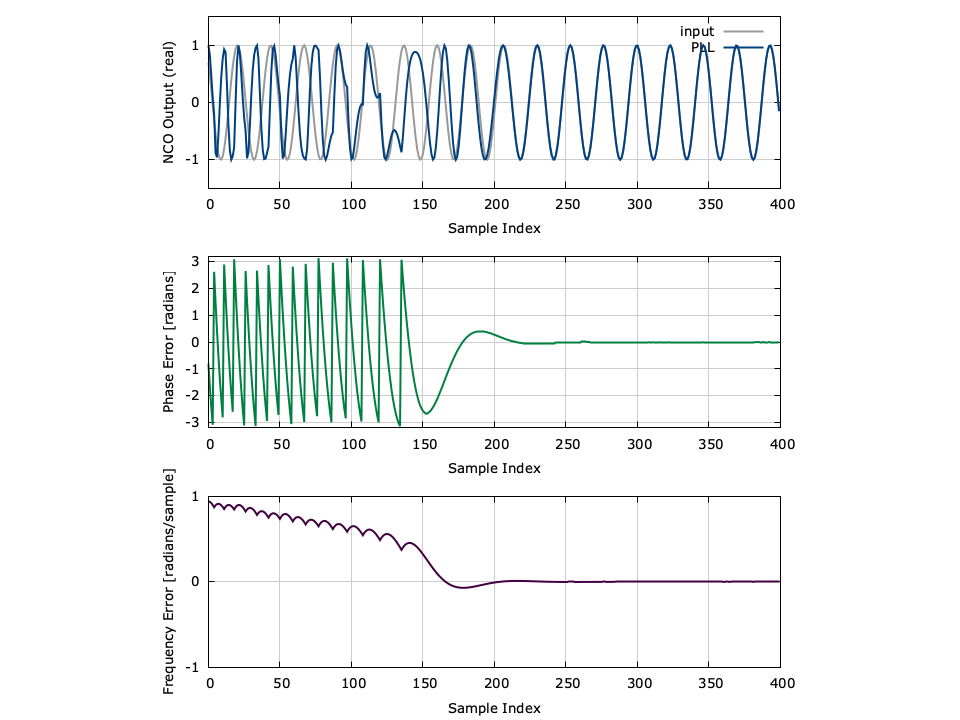
Figure [fig-nco-pll]. nco phase-locked loop demonstration
An example of the PLL can be seen in [ref:fig-nco-pll] . Notice that during the first 150 samples the NCO's output signal is misaligned to the input; eventually, however, the PLL acquires the phase of the input sinusoid and the phase error of the NCO's output approaches zero.