Linear Modem Bit Error Rates, Part II: Derivation
By  on February 28, 2015
Keywords: modulation modem bit error rate BER simulation
In this two-part tutorial I describe how to derive and simulate bit error rates for several linear modulation schemes. Part I of this tutorial explained how to simulate bit error rates for linear modulation schemes using the C programming language and [ref:liquid-dsp] . Part II derives the theoretical bit error rates values for several common modems.
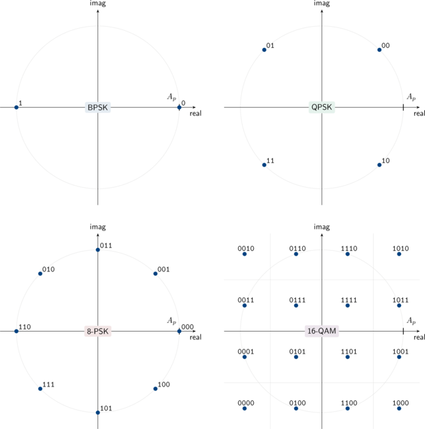
Figure [constellations]. Common linear digital modulation schemes with an average pulse amlitude \(A_p\)
Problem Statement∞
Part I of this tutorial provided a basic overview of linear modulation. Figure [ref:constellations] above depicts the constellation diagram of some common linear digital modulation schemes used in modern communications systems. Note that each point on the constellation represents a unique set of bits. Given an information message \(k \in \{0,1,\ldots,M-1\}\) , the transmitted symbol at complex baseband is the complex value \(s_k\) in the set \(\mathcal{S}_M = \{s_0,s_1,\ldots,s_{M-1}\}\) . For instance, if the information message is \(k=2\) for quadrature phase-shift keying, ( 10 binary), then the transmitted QPSK symbol would be \(s_2 = (1 - j)A_p/\sqrt{2}\) . Assuming perfect timing and carrier recovery the received sample will typically be the transmitted symbol with additional noise:
$$ r = s_k + n $$Under typical situations (the noise is uncorrelated, all symbols are equally likely to be used, etc.) the receiver's best guess at the transmitted symbol will be the one which is closest to the received sample. That is, linear modems demodulate by finding the closest of \(M\) symbols in the set \(\mathcal{S}_M\) to the received symbol \(r\) , viz
$$ \hat{s}_k = \underset{s_k \in \mathcal{S}_M}{\arg\min}\bigl\{ \| r - s_k \| \bigr\} $$For example, if the received sample \(r\) falls in the lower right quadrant of the QPSK constellation in the figure above, the receiver will assume the transmitted symbol was\(s_2\) and that the message was 10 .
Deriving the Bit Error Rate for BPSK∞
A common metric for evaulating the performance of a particular modulation scheme is to measure the theoretical bit error rate at the receiver. The bit error rate (BER) is dependent upon many factors, such as the modulation constellation, the signal and noise powers, and the noise distribution. By far the most common distribution used to model additive white noise is the Gauss (normal) distribution. The Gauss distribution's probability density and cumulative distribution functions are shown with a mean of zero and a standard deviation \(\sigma\) in the figures below.
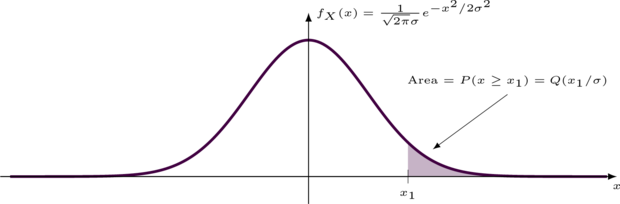
Figure [gauss_pdf]. Gauss Probability Density Function
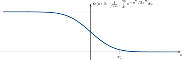
Figure [gauss_cdf]. Gauss Cumulative Density Function
One of the simplest and most common modulation schemes used is binary phase-shift keying (BPSK) which simply sends one of two pulses with equal amplitudes \(A_p\) :
$$ s_k = \begin{cases} +A_p & k=0 \\ -A_p & k=1 \end{cases} $$The transmitted signal is \(s = \pm A_p\) and the received signal under additive white Gauss noise is therefore
$$ \begin{array}{lll} r & = & s + n \\ & = & \pm A_p + \frac{1}{\sqrt{2\pi}\sigma}e^{-x^2/2\sigma^2} \end{array} $$Let's assume that the message is \(k=1\) and thus the transmitted signal\(s = s_1 = -A_p\) .
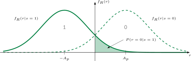
Figure [bpsk_distribution]. Binary phase-shift keying received signal distribution under additive white Gauss noise
The received value \(r\) will follow a Gauss distribution centered at \(-A_p\) as shown in Figure [ref:bpsk_distribution] with the solid green line. The symbol error probability (the probability of sending e.g. a 1 and receiving a 0 ) is just the probability that the noise is greater than \(A_p\) :
$$ \begin{array}{lll} P(r=0|s=1) & = & \int\limits_{0}^{\infty}{f_R(r=0|s=1)} \\ & = & \frac{1}{\sqrt{2\pi}\sigma}\int\limits_{0}^{\infty}{e^{-(u+A_p)^2/2\sigma^2} du} \\ & = & \frac{1}{\sqrt{2\pi}\sigma}\int\limits_{A_p}^{\infty}{e^{-u^2/2\sigma^2} du} \\ & = & Q\left(\frac{A_p}{\sigma}\right) \end{array} $$Because of symmetry and assuming that sending a 0 is as equally likely as sending a 1 , the symbol error probability is
$$ P_s = P(r=0|s=1) = Q\left(\frac{A_p}{\sigma}\right) $$The energy per symbol is just the variance of the symbol amplitude,\(E_s = A_p^2\) . The baseband noise power spectral density is related to its distribution's standard deviation as \(N_0/2 = \sigma^2\) . Therefore the signal-to-noise ratio (SNR) \(\gamma\) is
$$ \gamma \triangleq E_s / N_0 = A_p^2 / 2 \sigma^2 $$Solving for \(A_p/\sigma\) gives the symbol error rate as a function of SNR:
$$ P_s^{(BPSK)}(\gamma) = Q\left( \sqrt{2 \gamma} \right) $$In general we are interested not in the symbol error rate but rather the bit error rate. For BPSK, which has just one bit per symbol, these values are the same:
$$ P_b^{(BPSK)}(\gamma) = P_s(\gamma) = Q\left(\sqrt{2\gamma}\right) $$Deriving the Bit Error Rate for QPSK∞
Deriving the bit error rate for modulation schemes involving the quadrature phase is a bit trickier because we are concerned with two components of the signal as well as two components of the noise. With BPSK the information was contained solely within the in-phase component of the transmitted baseband signal.
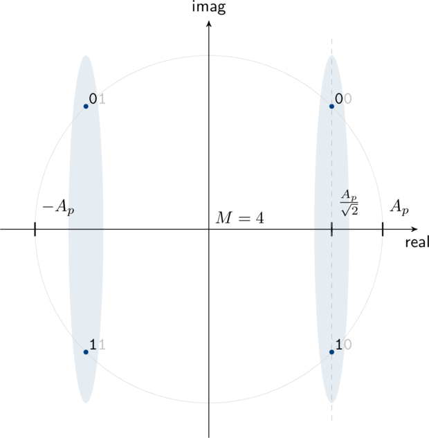
Figure [modem_qpsk_diagram]. Example demodulation region for QPSK
As its name might suggest, quadrature phase-shift keying (QPSK) uses both the in-phase and the quadrature components of the carrier signal to convey information, as can be seen in Figure [ref:modem_qpsk_diagram] . Doing so provides twice the information rate as BPSK, but at the cost of an increased error rate for the same signal-to-noise ratio because the symbols are now only separated by \(\sqrt{2} A_p\) instead of\(2 A_p\) as with BPSK. However QPSK can be considered in effect two BPSK signals in phase quadrature (see the highlighted sections in Figure [ref:modem_qpsk_diagram] ). That is, one bit is conveyed using the in-phase component of the carrier (the cosine) while the other bit is conveyed using the quadrature phase (the sine component). Because cosine and sine are orthogonal, there is in effect no interference between them (again, assuming perfect timing and carrier recovery). The only modification to the bit error rate computation is to compensate for the pulse scaling; that is, the energy for each component is now no longer \(A_p^2\) as with BPSK but
$$ E_s^{(QPSK)} = \left(\frac{A_p}{\sqrt{2}}\right)^2 = \frac{A_p^2}{2} $$Therefore the bit error rate for QPSK is the same as BPSK but with twice the power requirement:
$$ P_b^{(QPSK)}(\gamma) = Q\left(\frac{2 A_p}{\sigma}\right) = Q(\sqrt{\gamma}) $$Deriving the Bit Error Rate for 8-PSK∞
While the bit error rates for BPSK and QPSK can be derived in closed form with just a few terms and with relative ease, this is in general not the case for higher-ordered linear modulation schemes. This is because we cannot trivially separate the in-phase and quadrature components as we could with BPSK and QPSK. The true bit error rate for any generic linear modulation scheme involves computing the definite integral of a bivariate Gauss distribution. For 8-PSK this involves a double integration over each demodulation region as shown in Figure [ref:modem_8psk_diagram] . This is in general not a trivial task. Rather than dig into the gritty details, I will present a good approximation for the the symbol error probability of M-level phase-shift keying, viz
$$ P_s^{(M-PSK)}(\gamma) \approx 2 Q\left(\sqrt{2\gamma} \sin\left(\frac{\pi}{M}\right)\right) $$However, we are generally more interested in the bit error rate \(P_b\) rather than the symbol error rate \(P_s\) . As is often the case, when a symbol error occurs it is likely to happen to a symbol adjacent to the one that was sent.
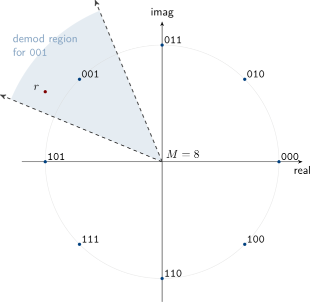
Figure [modem_8psk_diagram]. Example demodulation region for 8-PSK
If we arrange our bits appropriately such that nearby symbols differ by only one bit as is done in Figure [ref:modem_8psk_diagram] , we can assume that a symbol error most often results in just a single bit error. This is known as Gray Coding . Because only one of the three bits per symbol is likely to be in error for each symbol error, the bit error rate for 8-PSK is
$$ P_b^{(8-PSK)}(\gamma) \approx \frac{2}{3} Q\left(\sqrt{2\gamma} \sin\left(\frac{\pi}{8}\right)\right) $$As it turns out, this is a very good approximation for moderately large SNR values and only provides a slightly optimistic approximation when the SNR is below 0 dB.
Deriving the Bit Error Rate for 16-QAM∞
While it might not seem immediately obvious, we can actually separate the in-phase and quadrature components of 16-QAM as we could with BPSK and QPSK to provide an exact solution.
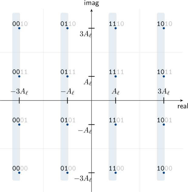
Figure [modem_16qam_diagram]. Example demodulation region for 16-QAM with the common in-phase bits highlighted
Figure [ref:modem_16qam_diagram] demonstrates that the first two bits of any symbol uniquely determine where the symbol's in-phase component is positioned. Consequently, the last two bits carry the quadrature information. As such, we can split the constellation into its two components and analyze them separately without loss of generatlity. The analysis for determining the exact bit error rate for 16-QAM follows in a similar way to that of QPSK . Consider the in-phase portion of the 16-QAM constellation in Figure [ref:modem_16qam_diagram] ; this is simply just a 4-level amplitude-shift keying (4-ASK) signal with two bits of information per symbol.
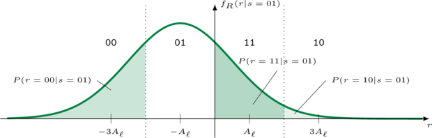
Figure [ask4_distribution]. 4-level amplitude-shift keying (4-ASK) under additive white Gauss noise
Figure [ref:ask4_distribution] depicts an example distribution of a received 4-ASK signal given that the transmitted message was \(k=1\) (and thus the transmitted symbol was \(s = s_1 = A_\ell\) ). Note that this is effectively the highlighted (in-phase) portion of Figure [ref:modem_16qam_diagram] . This is almost identical to the BPSK example in Figure [ref:bpsk_distribution] , except that there are one of 4 possible symbols instead of just 2. The thick green line denotes the probability of having received the value \(r\) given that the transmitted symbol was 01 . If an error occurred at the receiver, it was because one of the remaining three possible symbols was received:
$$ \begin{array}{lll} P(r=00|s=01) & = & Q\left( \frac{A_\ell}{\sigma}\right) \\ P(r=11|s=01) & = & Q\left( \frac{A_\ell}{\sigma}\right) - Q\left(3\frac{A_\ell}{\sigma}\right) \\ P(r=10|s=01) & = & Q\left(3\frac{A_\ell}{\sigma}\right) \end{array} $$We can now determine the probability of receiving a bit error given that the transmitted message was 01 by weighting the symbol errors by the number of bits that differ between each symbol and 01 :
$$ \begin{array}{lll} P(\mathrm{bit\,error}|s=01) & = & 1 \cdot Q\left( \frac{A_\ell}{\sigma}\right) \\ & + & 1 \cdot \left[ Q\left( \frac{A_\ell}{\sigma}\right) - Q\left(3\frac{A_\ell}{\sigma}\right)\right] \\ & + & 2 \cdot Q\left(3\frac{A_\ell}{\sigma}\right)\\ & = & 2 Q\left(\frac{A_\ell}{\sigma}\right) + Q\left(3\frac{A_\ell}{\sigma}\right) \end{array} $$We may similarly derive the bit error rates for sending the symbols 00 , 11 , and 10 respectively:
$$ \begin{array}{lll} P(\mathrm{bit\,error}|s=00) & = & Q\left(\frac{A_\ell}{\sigma}\right) + Q\left(3\frac{A_\ell}{\sigma}\right) - Q\left(5\frac{A_\ell}{\sigma}\right) \\ P(\mathrm{bit\,error}|s=11) & = & 2 Q\left(\frac{A_\ell}{\sigma}\right) + Q\left(3\frac{A_\ell}{\sigma}\right) \\ P(\mathrm{bit\,error}|s=10) & = & Q\left(\frac{A_\ell}{\sigma}\right) + Q\left(3\frac{A_\ell}{\sigma}\right) - Q\left(5\frac{A_\ell}{\sigma}\right) \end{array} $$To compute the bit error rate for 16-QAM, we need to relate the ratio\(A_\ell/\sigma\) to the signal to noise ratio \(\gamma\) . As before, we can compute the average symbol energy as the variance of the symbol amplitude,
$$ \begin{array}{lll} E_s^{(16-QAM)} & = & E\left\{s_k^2\right\} \\ & = & \frac{A_\ell^2}{16}\Bigl\{|1+j1|^2 + |1+j3|^2 + |3+j1|^2 + |3+j3|^2 + \cdots\Bigr\} \\ & = & 10 A_\ell^2 \end{array} $$If the one-sided noise power spectral density is \(\sigma = N_0/2\) , the signal-to-noise ratio is \(\gamma = E_s/N_0 = 10 A_\ell^2/2 \sigma\) , and therefore \(A_\ell/\sigma = \sqrt{\gamma/5}\) . The true bit error rate for 16-QAM is therefore
$$ P_b^{(16-QAM)} (\gamma) = \frac{3}{4} Q\left( \sqrt{\frac{\gamma}{5}} \right) + \frac{1}{2} Q\left( 3 \sqrt{\frac{\gamma}{5}} \right) - \frac{1}{2} Q\left( 5 \sqrt{\frac{\gamma}{5}} \right) $$Comparison to Simulation∞
Figure [ref:ber-comparison] below demonstrates the theorical bit error rates for BPSK, QPSK, 8-PSK, and 16-QAM as compared to simulation. Notice that while the 8-PSK bit error rate computation is only an approximation and provides a lower bound for the simulation, the values are nearly indistinguishable above an SNR of just 6 dB. All other computations are exact.
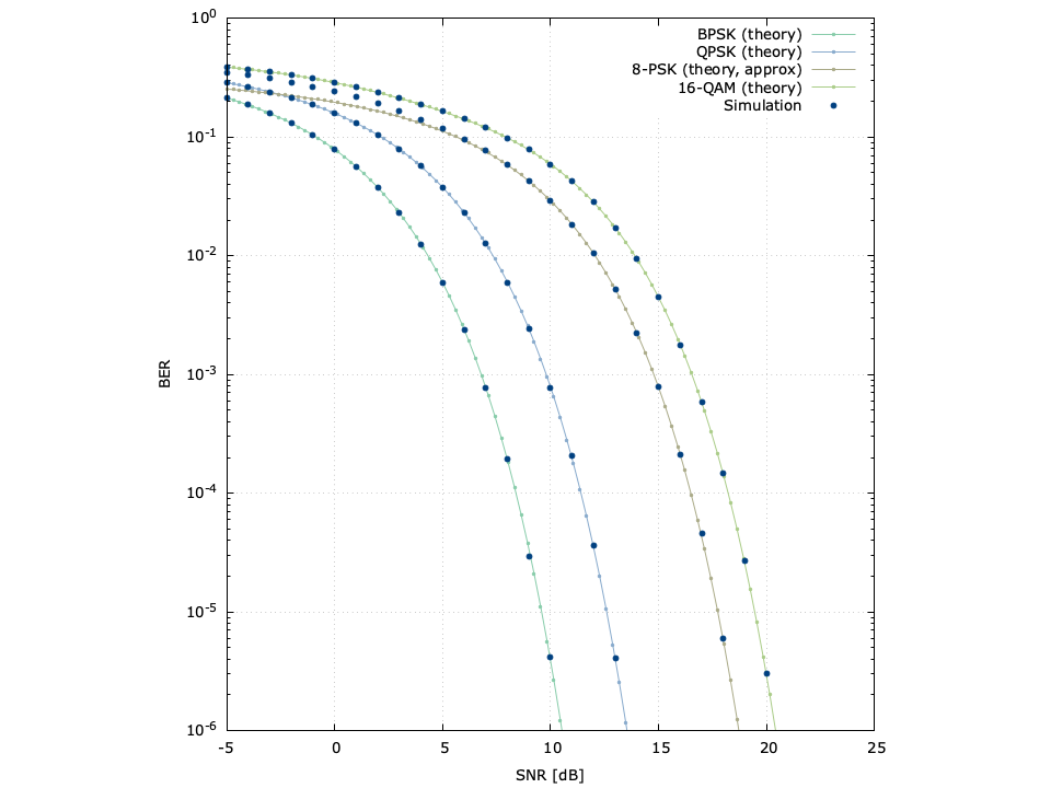
Figure [ber-comparison]. Comparison of simulation bit error rates to theoretical
For instructions on generating figures like the one above read Part I of this tutorial.